For gt_pca, the following types of plots are available:
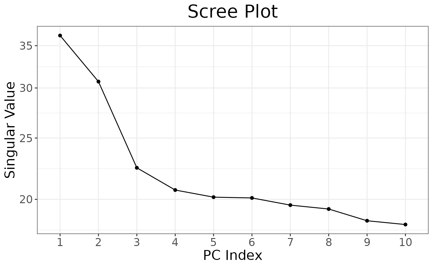
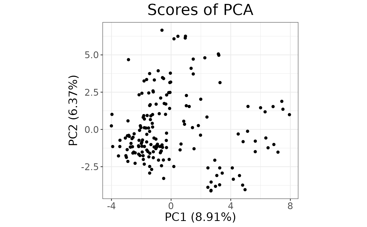
screeplot: a plot of the eigenvalues of the principal components (currently it plots the singular value)scoresa scatterplot of the scores of each individual on two principal components (defined bypc)loadingsa plot of loadings of all loci for a given component (chosen withpc)
Details
autoplot produces simple plots to quickly inspect an object. They are not
customisable; we recommend that you use ggplot2 to produce publication
ready plots.
Examples
library(ggplot2)
# Create a gen_tibble of lobster genotypes
bed_file <-
system.file("extdata", "lobster", "lobster.bed", package = "tidypopgen")
lobsters <- gen_tibble(bed_file,
backingfile = tempfile("lobsters"),
quiet = TRUE
)
# Remove monomorphic loci and impute
lobsters <- lobsters %>% select_loci_if(loci_maf(genotypes) > 0)
lobsters <- gt_impute_simple(lobsters, method = "mode")
# Create PCA object
pca <- gt_pca_partialSVD(lobsters)
# Screeplot
autoplot(pca, type = "screeplot")
 # Scores plot
autoplot(pca, type = "scores")
# Scores plot
autoplot(pca, type = "scores")
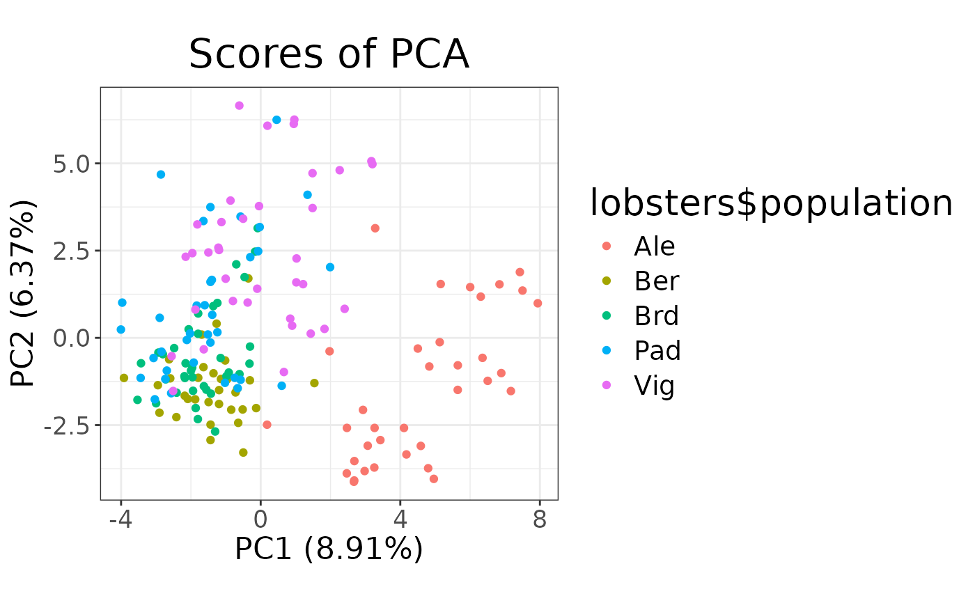
 # Colour by population
autoplot(pca, type = "scores") + aes(colour = lobsters$population)
# Colour by population
autoplot(pca, type = "scores") + aes(colour = lobsters$population)
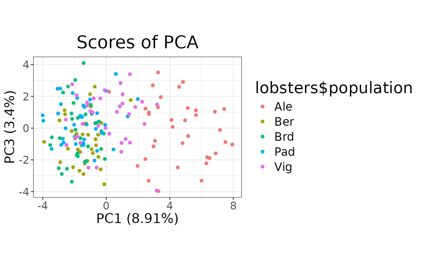
 # Scores plot of different components
autoplot(pca, type = "scores", k = c(1, 3)) +
aes(colour = lobsters$population)
# Scores plot of different components
autoplot(pca, type = "scores", k = c(1, 3)) +
aes(colour = lobsters$population)