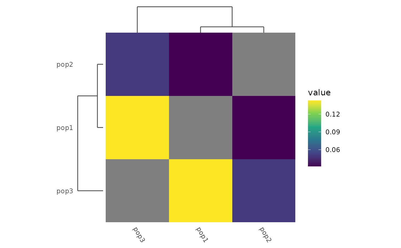
Add dendrograms to a heatmap of pairwise distances

This function adds dendrograms to a heatmap of pairwise distances, generated with heatmap_pairwise(). The heatmap must have been created with an order function based on hclust(), and the dendrograms will be based on the same clustering. Dendrograms can be added to the left (row) and/or top (column) of the heatmap. Note that the heatmap needs to be formatted first, as it can not be modified easily once the dendrogram panels have been added.

Usage

heatmap_add_dendro(
  plot,
  side = c("both", "left", "top"),
  rel_size = 0.15,
  line_color = "grey30",
  line_size = 0.5
)

Arguments

plot

A ggplot from heatmap_pairwise(), with an order function based on hclust().

side

"left" (row dendrogram), "top" (column dendrogram), or "both".

rel_size

Size of the dendrogram relative to the panel (null unit).

line_color

Segment colour.

line_size

Segment linewidth.

Value

A heatmap_dendro object (a subclass of gtable), which auto-draws on print() and is accepted by plot() and ggsave(), just like a ggplot or patchwork object.

Details

To correctly align the dendrogram with the labels of the heatmap, we use a gtable to insert the dendrogram panel directly adjacent to the heatmap panel. This means that the dendrogram will be perfectly aligned with the heatmap cells regardless of axis label width. However, manipulating individual plots in a gtable is not easy, so the heatmap should be formatted fully before the dendrograms are added.

Examples

example_gt <- load_example_gt("gen_tbl")
# With a pairwise matrix:
fst_dist <- example_gt %>%
  group_by(population) %>%
  pairwise_pop_fst(method = "Nei87", type = "pairwise")
mat_plot <- heatmap_pairwise(fst_dist,
  order = function(x) {
    stats::hclust(stats::as.dist(x))
  }) +
ggplot2::scale_fill_viridis_c()
heatmap_add_dendro(mat_plot)