Georeference an image
georeference_image.RmdGeoreferencing is the process of assigning real-world coordinates to
an image, allowing it to be accurately placed on a map. This is often
done using Ground Control Points (GCPs), which are known locations on
the ground with precise coordinates. In this vignette, we will
demonstrate how to georeference an image using GCPs in the
crstools package.
The process of assigning GCPs to an image is interactive, allowing
you to select points on the image and assign them geographic
coordinates. Unfortunately, this is not compatible with Rmarkdown or the
image pane within RStudio. crstools opens separate windows
for GCP assignment and image display, and the code has to be run from a
script or the console.
To get started, we need to load the crstools
package:
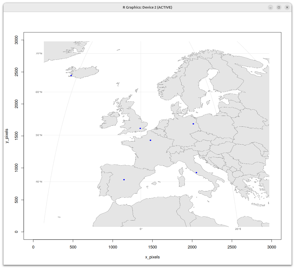
library(crstools)Next we need a .jpg image that we scanned or downloaded. We will use a map of Europe that is included with the package. The map has a number of points (the capitals of UK, France, Spain, Germany, Italy, and Iceland).
Our task is to georeference this image and then extract the coordinates of those capitals. We will copy a version of the image to a temporary directory, and work on that:
file.copy(
  from = system.file("extdata/europe_map.jpeg", package = "crstools"),
  to = tempdir(),
  overwrite = TRUE
)
#> [1] TRUE

img_path <- file.path(tempdir(), "europe_map.jpeg")
We can now select a number of GCPs with choose_gcp().
This function allows you to click on the image and assign coordinates to
the points you select. Choose locations that are easy to find again on a
map, such as features in coastlines (e.g. bays), or corners of country
boundaries.
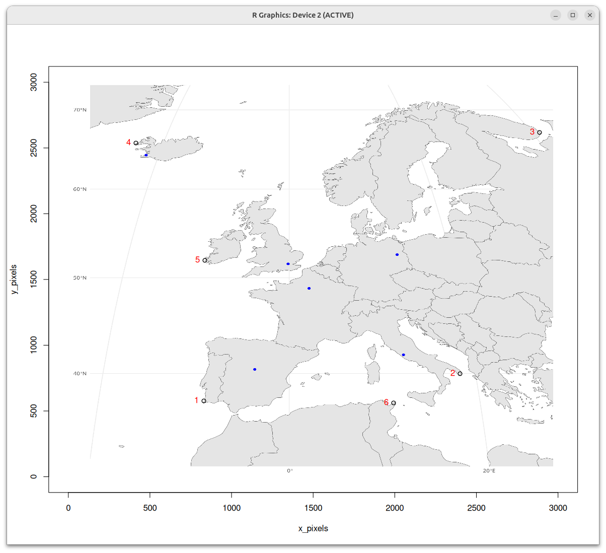
gcp_europe <- choose_gcp(img_path)This will open a window showing the image:
choose_gcp()
You can click on the image to select points by left-clicking with your mouse. The points will be numbered in the order in which they were chosen; you can stop by pressing the ESC key, or with a right-click.
The coordinates of those points will be saved in the
gcp_europe dataframe, which contains the following
columns:
gcp_europe
#>   id         x         y longitude latitude
#> 1  1  830.3113  576.5869        NA       NA
#> 2  2 2399.7464  783.3988        NA       NA
#> 3  3 2886.9187 2617.8971        NA       NA
#> 4  4  414.0564 2537.4702        NA       NA
#> 5  5  836.4781 1645.1151        NA       NA
#> 6  6 1992.7416  561.2675        NA       NA
Next we need to get the coordinates (longitude and latitude) of these
points. We can use the find_gcp_coords() function to assign
geographic coordinates to the GCPs. This function requires a reference
map in the form of an sf object. We will use the
rnaturalearth package to get a map of Europe, and then crop
it to the extent of the image.
library(sf)
#> Linking to GEOS 3.12.1, GDAL 3.8.4, PROJ 9.4.0; sf_use_s2() is TRUE
library(rnaturalearth)
# Load the world map
world <- ne_countries(scale = "medium", returnclass = "sf")
# Transform it to a suitable projection
world <- st_transform(world, crs = 4326) # WGS 84
# Crop it to the extent of the image to Europe
europe <- st_crop(world, c(xmin = -25, ymin = 25, xmax = 45, ymax = 70))
#> Warning: attribute variables are assumed to be spatially constant throughout
#> all geometries
Let’s quickly plot it to check that we have the correct extent:
library(ggplot2)
ggplot() +
  geom_sf(data = europe, fill = "lightblue", color = "black") +
  coord_sf(expand = FALSE) +
  ggtitle("Map of Europe")
Now we can use the find_gcp_coords() function to assign
geographic coordinates to the GCPs.
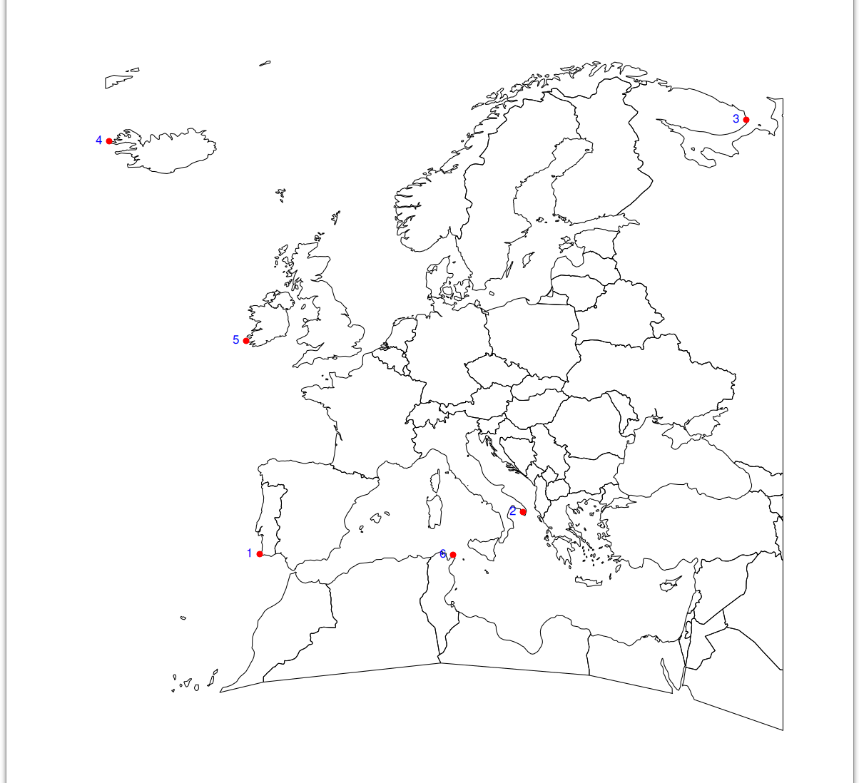
find_gcp_coords()
gcp_europe_coords <- find_gcp_coords(gcp_europe, europe)This will open a new window with the map of Europe, and you can click on the points to assign coordinates to the GCPs.
Now the gcp_europe_coords dataframe contains the
geographic coordinates of the GCPs:
gcp_europe_coords
#>   id         x         y  longitude latitude
#> 1  1  830.3113  576.5869  -9.071636 37.16461
#> 2  2 2399.7464  783.3988  18.132085 40.06647
#> 3  3 2886.9187 2617.8971  41.207327 67.11767
#> 4  4  414.0564 2537.4702 -24.627151 65.64215
#> 5  5  836.4781 1645.1151 -10.472369 51.87063
#> 6  6 1992.7416  561.2675  10.907249 37.11543
Finally, we can use the georeference_image() function to
georeference the image using the GCPs. This function will create a new
TIFF file with the georeferenced image.
georeferenced_image <- georeference_img(img_path, gcp_europe_coords)The georeference_img() function will create a new TIFF
file with the georeferenced image. The output file will have the same
name as the input image, but with the suffix _warp.tif
added to it.
The georeferenced image can be loaded into R using the
terra package as a SpatRaster:
map_warp <- terra::rast(georeferenced_image)We can now plot the georeferenced image to check the overlap between
the input image and the georeferenced image. This can inform us if more
points (GCPs) need to be added and previous steps repeated
(choose_gcp()).
library(ggplot2)
library(tidyterra)
ggplot() +
  geom_spatraster_rgb(data = map_warp) +
  geom_sf(
    data = europe,
    color = "orange",
    fill = "transparent"
  ) +
  coord_sf(expand = FALSE)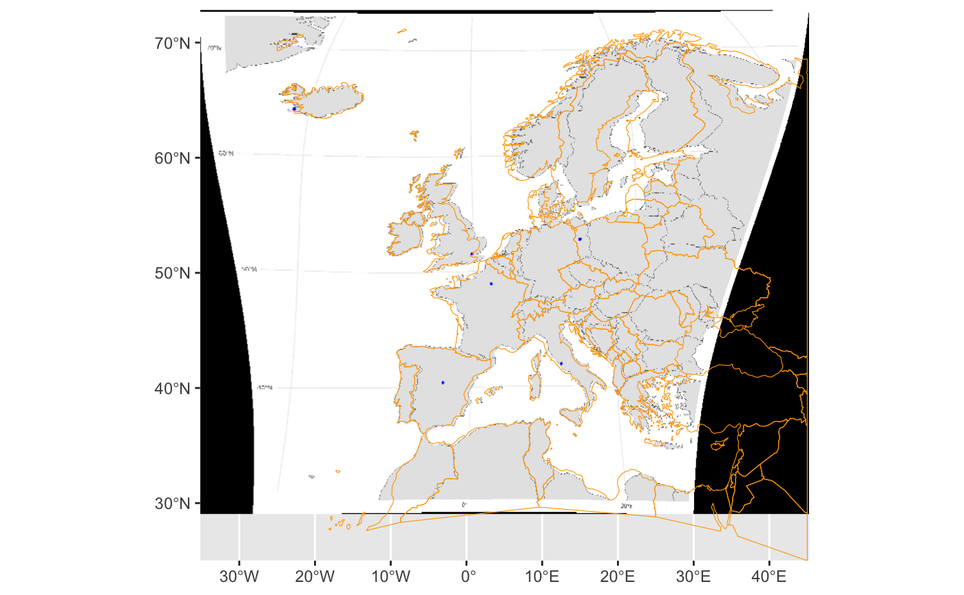
To add more points to improve the fit, we use:
gcp_europe <- choose_gcp(img_path, gcp = gcp_europe)Additional points were added to the gcp_europe
dataframe:
gcp_europe
#>    id         x         y longitude latitude
#> 1   1  830.3113  576.5869        NA       NA
#> 2   2 2399.7464  783.3988        NA       NA
#> 3   3 2886.9187 2617.8971        NA       NA
#> 4   4  414.0564 2537.4702        NA       NA
#> 5   5  836.4781 1645.1151        NA       NA
#> 6   6 1992.7416  561.2675        NA       NA
#> 7   7 2641.4229  246.7386        NA       NA
#> 8   8 2576.9680  632.6570        NA       NA
#> 9   9 2377.7439 2189.4124        NA       NA
#> 10 10 2190.2389 2457.5930        NA       NA
#> 11 11 2172.6603 2156.7075        NA       NA
#> 12 12 2108.2054 1960.4778        NA       NA
#> 13 13 1826.9479 2032.4287        NA       NA
#> 14 14 1668.7405 2065.1336        NA       NA
#> 15 15 1112.0849 1417.5757        NA       NA
#> 16 16 1258.5732 2032.4287        NA       NA
Check the map with the original points

Now we can repeat the process of assigning coordinates to the GCPs
using find_gcp_coords() and
georeference_img():
gcp_europe_coords_v2 <- find_gcp_coords(gcp_europe, europe)

gcp_europe_coords_v2
Run the following code chunk to save the object if you are recreating the vignette
Repeat georeferencing of the image using the GCPs
georeferenced_image_v2 <- georeference_img(img_path, gcp_europe_coords_v2)

map_warp_v2 <- terra::rast(georeferenced_image_v2)

# check the new image
ggplot() +
  geom_spatraster_rgb(data = map_warp_v2) +
  geom_sf(
    data = europe,
    color = "orange",
    fill = "transparent"
  ) +
  coord_sf(expand = FALSE)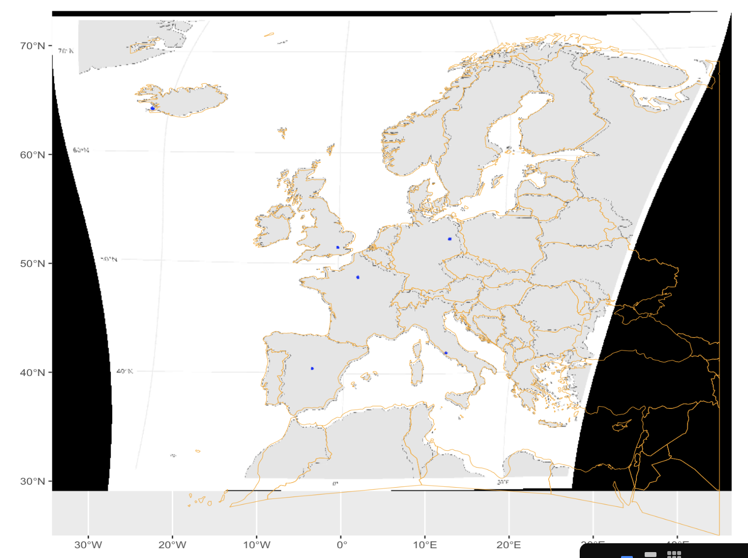
We can see that the additional points improved the georeferencing of the image, as the map now aligns better with the geographic coordinates of the GCPs.
We now use locator to get the coordinates of the blue dots
# get the coordinates of the blues points
blue_coords_df <- extract_coords(map_warp_v2)
So we now have the coordinates of the blue dots:
blue_coords_df
#>   id   longitude latitude
#> 1  1  -3.2609722 40.36582
#> 2  2  12.5085660 41.72656
#> 3  3  12.9900786 52.31006
#> 4  4  -0.4922746 51.47850
#> 5  5 -22.4010987 64.17870
There are only 5 entries - we forgot one of the dots, let’s re run the function:
blue_coords_df <- extract_coords(map_warp_v2, blue_coords_df)So we now we can see check that all the blue dots have been recorded:
blue_coords_df
#>   id   longitude latitude
#> 1  1  -3.2609722 40.36582
#> 2  2  12.5085660 41.72656
#> 3  3  12.9900786 52.31006
#> 4  4  -0.4922746 51.47850
#> 5  5 -22.4010987 64.17870
#> 6  6   1.9152885 48.68143
Starting from a non georeferenced image, we were then able to extract the coordinates of our locations of interest.