Projection of aDNA samples onto modern PCA
2024-06-12
Source:vignettes/articles/pca_aDNA_projection.Rmd
pca_aDNA_projection.RmdThe following article shows how to project ancient DNA data onto
modern data in a Principal Components Analysis using the
tidypopgen package.
The example uses the data from Lazaridis et al. (2016). After
downloading the data in PACKEDANCESTRYMAP format files, we convert them
into gen_tibble objects. This vignette replicates the
workflow illustrated in the vignette for the R package
smartsnp, but works directly on
gen_tibbles.
First, we can download the data from the Reich lab website.
Download the data
temp_dir <- tempdir()
# Download file using R's download.file function
download_url <- "https://reich.hms.harvard.edu/sites/reich.hms.harvard.edu/files/inline-files/NearEastPublic.tar.gz"
download_path <- file.path(temp_dir, "NearEastPublic.tar.gz")
download.file(download_url, download_path, mode = "wb")
We can then move and extract our data into a folder called
data/.
+# Create data directory
if (!dir.exists("data")) dir.create("data")
if (!dir.exists("data/NearEastPublic")) dir.create("data/NearEastPublic")
# Copy downloaded file
file.copy(download_path, "data/NearEastPublic.tar.gz")
# Extract using R's untar function
utils::untar("data/NearEastPublic.tar.gz", exdir = "data/NearEastPublic")
Read in the data
Now that our data are downloaded, we can use tidypopgen
to read the data into gen_tibble objects, beginning with
the modern data:
HO_modern <- gen_tibble("./data/NearEastPublic/HumanOriginsPublic2068.geno",
                        quiet = TRUE,
                        backingfile = tempfile("test_"))
Followed by the ancient data:
ancient <- gen_tibble("./data/NearEastPublic/AncientLazaridis2016.geno",
                      quiet = TRUE,
                      backingfile = tempfile("test_"))
Subset modern data
For our analysis, we will be projecting ancient European individuals,
so we only need modern West Eurasian populations. We can select these
populations by filtering the gen_tibble object using the
filter() function from the dplyr package:
westEurasian_pops <- c(
  "Abkhasian", "Adygei", "Albanian", "Armenian", "Assyrian", "Balkar", "Basque", "BedouinA", "BedouinB", "Belarusian", "Bulgarian", "Canary_Islander",
  "Chechen", "Croatian", "Cypriot", "Czech", "Druze", "English", "Estonian", "Finnish", "French", "Georgian", "German", "Greek", "Hungarian", "Icelandic",
  "Iranian", "Irish", "Irish_Ulster", "Italian_North", "Italian_South", "Jew_Ashkenazi", "Jew_Georgian", "Jew_Iranian", "Jew_Iraqi", "Jew_Libyan", "Jew_Moroccan",
  "Jew_Tunisian", "Jew_Turkish", "Jew_Yemenite", "Jordanian", "Kumyk", "Lebanese_Christian", "Lebanese", "Lebanese_Muslim", "Lezgin", "Lithuanian", "Maltese",
  "Mordovian", "North_Ossetian", "Norwegian", "Orcadian", "Palestinian", "Polish", "Romanian", "Russian", "Sardinian", "Saudi", "Scottish", "Shetlandic", "Sicilian",
  "Sorb", "Spanish_North", "Spanish", "Syrian", "Turkish", "Ukrainian"
)

HO_modern <- HO_modern %>% filter(HO_modern$population %in% westEurasian_pops)
Create Modern PCA
Before we run a PCA on the modern Eurasian individuals, we need to impute any missing genotypes.
As we have subset our gen_tibble object, first we need
to update our backingfile to this subset:
HO_modern <- gt_update_backingfile(HO_modern,
                                   quiet = TRUE)
And then we can impute, using:
HO_modern <- gt_impute_simple(HO_modern, method = "mean")We should also remove any monomorphic loci from our data, as these
loci are uninformative. Monomorphic markers must always be removed
before a PCA is computed using any of the gt_pca
functions.
To do this, we use the select_loci_if function together
with loci_maf to select only genotypes where MAF is greater
than 0:
HO_modern <- HO_modern %>% select_loci_if(loci_maf(genotypes)>0)Now we can create our PCA object from the modern data:
pca <- gt_pca_partialSVD(HO_modern, k = 2)We can then use augment to add the PCA coordinates for
each individual to our gen_tibble object:
HO_modern_pca <- augment(x = pca, data = HO_modern, k = 2)Projection
Before projecting, we remove ancient individuals and outgroups that are not of interest:
# Samples to remove:
sample.rem <- c("Mota", "Denisovan", "Chimp", "Mbuti.DG", "Altai",
               "Vi_merge", "Clovis", "Kennewick", "Chuvash", "Ust_Ishim",
               "AG2", "MA1", "MezE", "hg19ref", "Kostenki14")

ancient <- ancient %>% filter(!ancient$population %in% sample.rem)
And now we can project our data using the predict
function:
predicted <- predict(object = pca, new_data = ancient, project_method = "least_squares")Here, we use the “least_squares” argument to generate a least squares
projection that will be comparable to the approach used in
smartpca (also implemented in the R package
smartsnp).
Finally, we can tidy up our data ready to plot by converting the
predicted object to a data frame and adding the population
names:
predicted <- as.data.frame(predicted)
predicted$id <- ancient$id
predicted$population <- ancient$population
Result
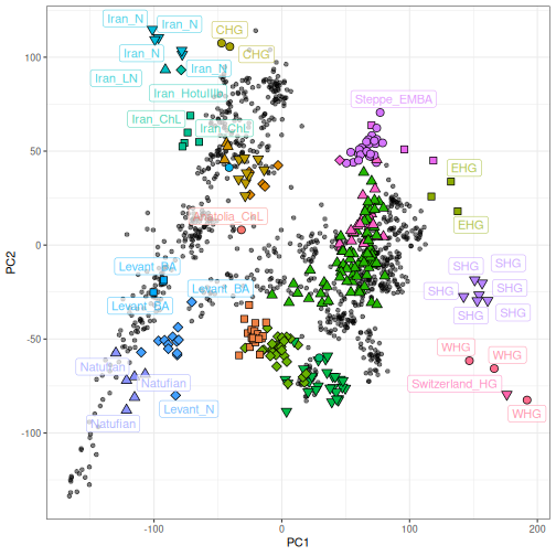
The PCA and predicted individuals can then be visualized using
ggplot2 by layering a geom of ancient individuals over
modern individuals, using the same syntax as smartsnp:
ggplot() +
  geom_point(data = HO_modern_pca, aes(x = .fittedPC1, y = .fittedPC2), alpha=0.5) +
  geom_point(data = predicted, aes(.PC1,.PC2, fill=population, shape=population), size=3) +
  scale_shape_manual(values=rep(21:25, 100)) +
  geom_label_repel(data = predicted, aes(.PC1,.PC2, label=population, col=population), alpha=0.7, segment.color="NA") +
  theme_bw() + theme(legend.position = "none")+
  labs(x = "PC1", y = "PC2")
## Warning: ggrepel: 247 unlabeled data points (too many overlaps). Consider increasing max.overlaps