This function estimates the home range of an animal using kernel density
estimation (KDE).
The home range is estimated for each group in x, which can be defined by
grouping x by one or more variables. If x is not grouped, the track ID
is used as grouping variable, and the home range is estimated for each track
separately.
Usage
hr_tt_kde(x, h = "h_ref_mean", bbox = NULL, res = NULL, levels = NULL)

hr_kde(x, h = "h_ref_mean", bbox = NULL, res = NULL, levels = NULL)
Arguments
- x
A move2 object; if explicitly grouped, the home range is estimated for each group, combining all tracks within each group. Otherwise, the track id is used as grouping variable.
- h
The bandwidth for the kernel density estimation. Either a number, or "h_ref_indiv" for using the reference bandwidth for each individual, or "h_ref_mean" for using the mean bandwidth for all individuals (the default).
- bbox
A named vector of four elements (
xmin,ymin,xmax,ymax) defining a grid shared by all groups, or a list of one such vector per group. IfNULL, a shared grid is created from the extent of all points inx, expanded by 100% of the range on each side.- res
The resolution of the grid (in the units of the projection of x). Supply one value for a shared resolution or one value per group when
bboxcontains one grid per group. IfNULL, each grid is assigned a resolution that produces approximately 1000 cells.- levels
A vector of levels for the isopleths (i.e. contour lines), as numbers between 0 and 1. If set to NULL (the default), the full utilisation distribution is returned; otherwise just the isopleths are returned. It is possible to specify more than two levels, e.g.
c(0.5, 0.95)corresponds to the 50% and 95% home ranges.
Value
Either a tibble, or, if levels is not NULL, an sf tibble ,
with columns:
the grouping variable (as named in
x; ifxis grouped by multiple variables, this column is namedgroup_id): the ids from the grouping ofxlevel: the level of the isoplethh: the bandwidth used for the KDExmin,ymin,xmax,ymax: the bounding box used for the KDEres: the resolution used for the KDE Iflevelsis NULL:ud: the full utilisation distribution is returned as a list-column ofterra::SpatRasterobjects Else, iflevelsis not NULL, the following columns are added:area: the area of the home range at this level (in the units of the projection ofx, e.g. m^2 for a UTM projection)geometry: ansfccolumn containing the multipolygons representing the isopleth for the appropriate level
Details
By default, the full UD is returned. If levels is set, the
isopleths for the specified levels are returned instead, along with their
area. This option is useful to reduce memory use, but has the drawback that
the full UD is not returned, which can be useful for some applications (e.g.
to compute overlap between home ranges). If levels is set, the area of the
isopleths is computed using sf::st_area(), which returns the area in the
units of the projection of x (e.g. m^2 for a UTM projection). If x is
unprojected, the area is computed in degrees^2, which is not a meaningful
unit for area. In this case, it is recommended to project x to an
appropriate projection before using this function.
Examples
example_kde <- hr_tt_kde(example_tt)
example_kde
#> # A tibble: 3 × 9
#> track_id method h xmin ymin xmax ymax res ud
#> <chr> <chr> <dbl> <dbl> <dbl> <dbl> <dbl> <dbl> <named list>
#> 1 a kde 1.06 -16.5 -7.42 16.6 9.54 0.737 <SpatRstr[,45,1]>
#> 2 b kde 1.06 -16.5 -7.42 16.6 9.54 0.737 <SpatRstr[,45,1]>
#> 3 c kde 1.06 -16.5 -7.42 16.6 9.54 0.737 <SpatRstr[,45,1]>
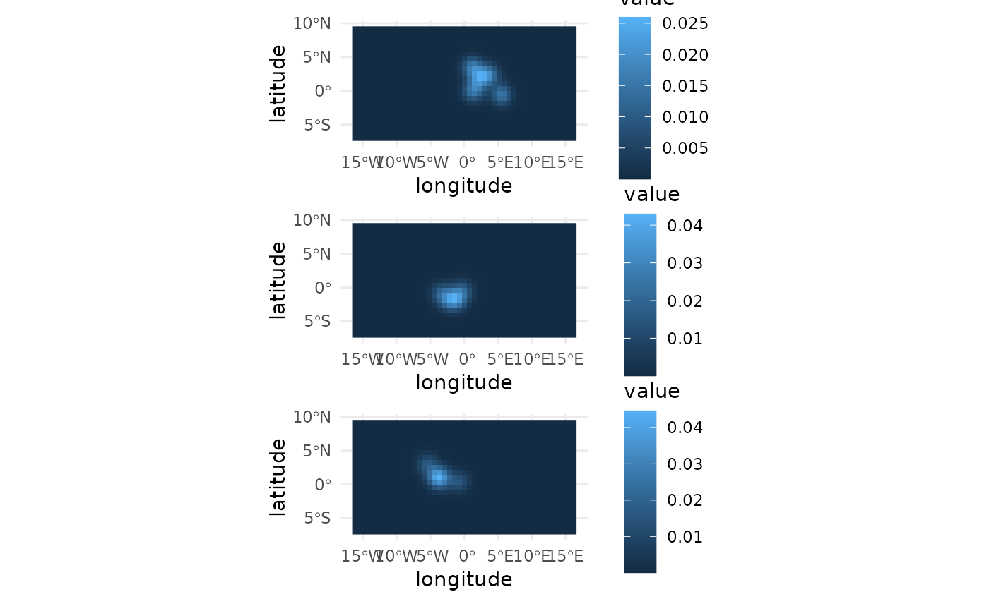
library(ggplot2)
autoplot(example_kde)
 # compute the isopleths for the 50% and 95% home range
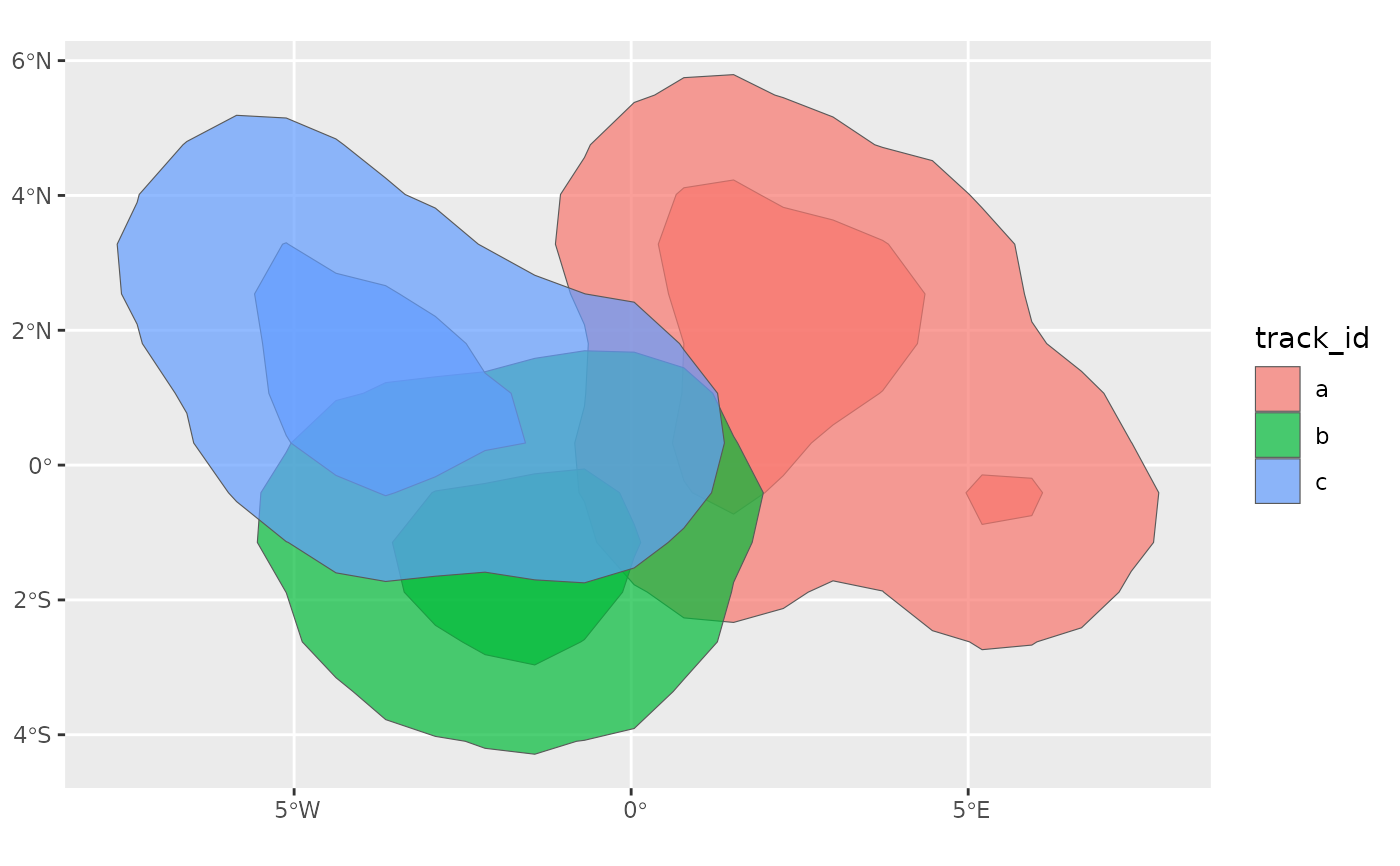
example_iso <- hr_tt_kde(example_tt, levels = c(0.5, 0.95))
ggplot(example_iso) +
geom_sf(aes(fill = track_id), alpha = 0.7)
# compute the isopleths for the 50% and 95% home range
example_iso <- hr_tt_kde(example_tt, levels = c(0.5, 0.95))
ggplot(example_iso) +
geom_sf(aes(fill = track_id), alpha = 0.7)