Quantify the home range using minimum convex polygon (MCP)

This function estimates the home range of an animal using the minimum convex polygon (MCP) method.

Usage

hr_tt_mcp(x, levels = c(0.5, 0.95))

hr_mcp(x, levels = c(0.5, 0.95))

Arguments

x: A move2 object; if explicitly grouped, the home range is estimated for each group, combining all tracks within each group. Otherwise, the track id is used as grouping variable.
levels: A vector of levels for the contour lines. The default is c(0.5, 0.95), which corresponds to the 50% and 95% home ranges.

Value

A tibble of subclass hr_tt_poly_tbl of results, with columns:

group_id: the ids from the grouping of x
level: the level of the contour line
geometry: the geometry of the home range as a list of sf polygons

Examples

example_mcp <- hr_tt_mcp(example_tt)
example_mcp
#> Simple feature collection with 6 features and 4 fields
#> Geometry type: POLYGON
#> Dimension:     XY
#> Bounding box:  xmin: -5.5053 ymin: -1.9431 xmax: 3.6119 ymax: 3.5288
#> Geodetic CRS:  WGS 84
#> # A tibble: 6 × 5
#>   track_id method level         area                                    geometry
#>   <chr>    <chr>  <dbl>        [m^2]                               <POLYGON [°]>
#> 1 a        mcp     0.95 52747834477. ((1.371 -0.0627, 1.1694 3.5288, 3.6119 2.3…
#> 2 a        mcp     0.5  14105533708. ((1.371 -0.0627, 2.2065 1.8612, 3.6119 2.3…
#> 3 b        mcp     0.95 13139194429. ((-0.9581 -1.5686, -1.427 -1.9431, -2.4405…
#> 4 b        mcp     0.5   2865637069. ((-1.427 -1.9431, -2.4405 -1.7632, -0.9581…
#> 5 c        mcp     0.95  6222600829. ((-3.8075 1.2897, -3.4103 0.8278, -4.0496 …
#> 6 c        mcp     0.5   1241642121. ((-3.4103 0.8278, -4.0496 1.0655, -3.8075 …
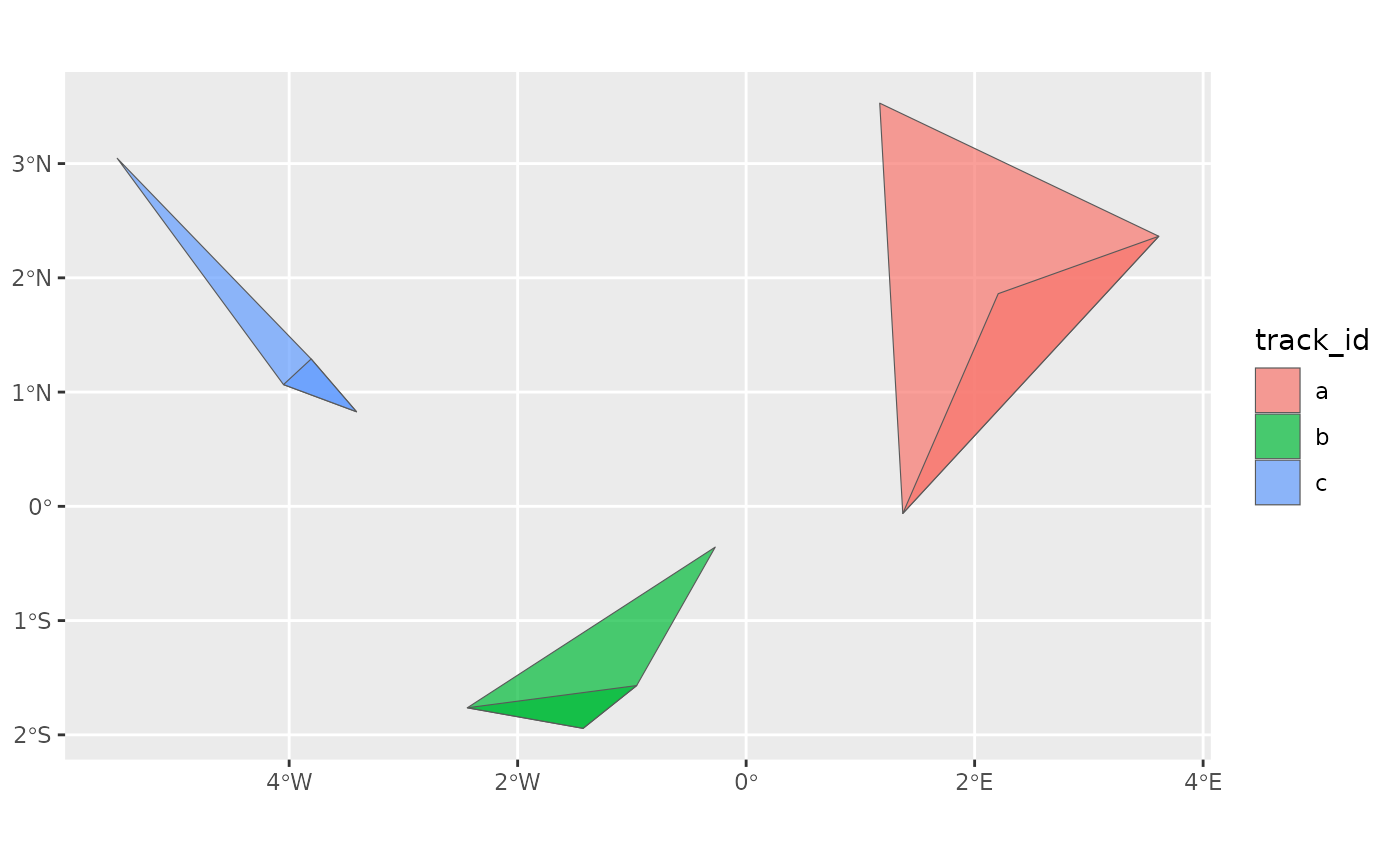
library(ggplot2)
ggplot(example_mcp) +
  geom_sf(aes(fill = track_id), alpha = 0.7)