The generic function buffer finds buffers around specified locations
of a gGraph or a gData object. Different format
for the output are available.
Details
The computed buffers are sets of nodes lying within a given distance of specified locations. All nodes of a buffer need to be connected to the location they surround.
Examples
#### gGraph example ####
## Subset gGraph to Europe
x <- rawgraph.10k[isInArea(worldgraph.10k, reg = list(x = c(-10, 50), y = c(35, 70)), quiet = TRUE)]
## identify one node
node <- closestNode(x, data.frame(lon = 12, lat = 50))
## find a buffer
buffer(x, node, 1000)
#> [1] "7377" "7057" "7697" "7378" "7376" "7056" "7698" "6737" "7058" "6736"
#> [11] "8017" "7696" "8018" "7379" "7699" "7375" "7055" "6735" "8019" "6417"
#> [21] "6738" "6416" "7059" "6415" "8337" "8016" "8338" "7695" "8339" "7380"
#> [31] "7700" "8020" "7374" "7054" "6734" "6414" "8340" "6097" "6418" "6096"
#> [41] "6739" "6095" "7060" "6094" "8657" "8336" "8658" "8015" "8659" "7694"
#> [51] "8660" "7381" "7701" "8021" "8341" "7373" "7053" "6733" "6413" "6093"
#> [61] "8661" "8022" "8342"
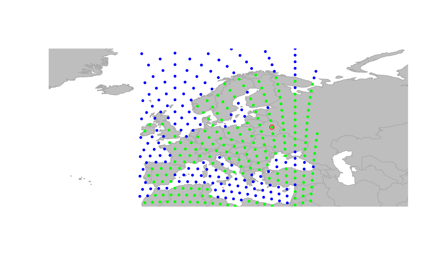
buf500km <- buffer(x, node, 1000, res.type = "gGraph")
plot(buf500km, col.rules = buf500km@meta$buf.colors, reset = TRUE)
#> Spherical geometry (s2) switched off
 #> Spherical geometry (s2) switched on
#### gData example ####
## retain a subset of hgdp
x <- hgdp[27:30]
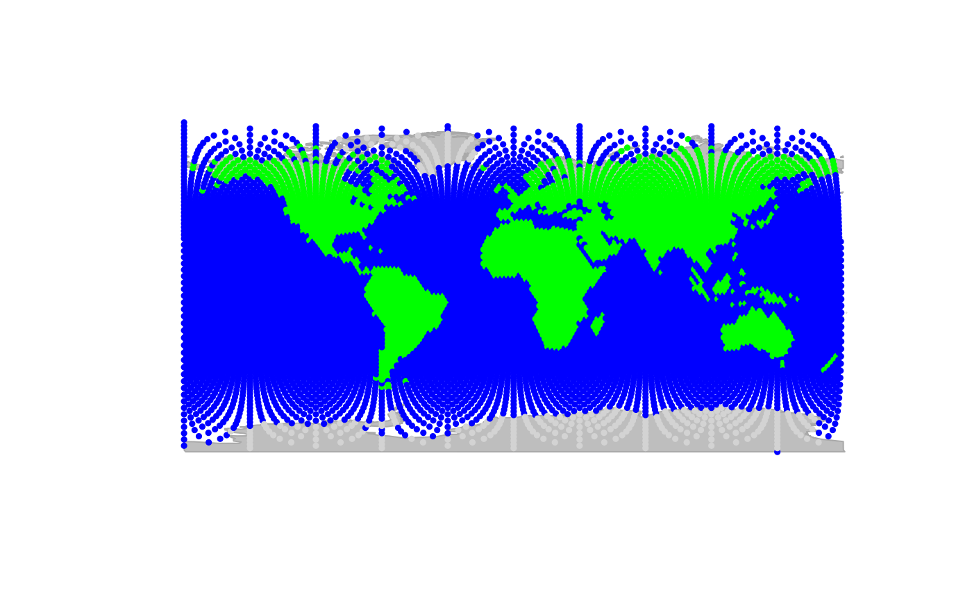
plot(x, reset = TRUE, col.g = "lightgrey", pch.node = 20)
#> Spherical geometry (s2) switched off
#> Spherical geometry (s2) switched on
buf.400 <- buffer(x, 400, res.type = "gData")
points(buf.400, col.node = "gold")
#> Spherical geometry (s2) switched on
#### gData example ####
## retain a subset of hgdp
x <- hgdp[27:30]
plot(x, reset = TRUE, col.g = "lightgrey", pch.node = 20)
#> Spherical geometry (s2) switched off
#> Spherical geometry (s2) switched on
buf.400 <- buffer(x, 400, res.type = "gData")
points(buf.400, col.node = "gold")