Examples of additional tidymodels features
Source:vignettes/a2_tidymodels_additions.Rmd
a2_tidymodels_additions.RmdIn this vignette, we illustrate how a number of features from
tidymodels can be used to enhance a conventional SDM
pipeline. If you’re new to tidymodels; there are a number
of excellent tutorials (both introductory and advanced) on its dedicated
website. We reuse the example
on the Iberian lizard from the tidysdm
overview article. Subsection are written to be self-contained, so
you can read and run them independently.
Using multi-level factors as predictors
Most machine learning algorithms do not natively use multilevel
factors as predictors. The solution is to create dummy variables, which
are binary variables that represent the levels of the factor. In
tidymodels, this is done using the step_dummy
function.
Let’s create a factor variable with 3 levels based on altitude.
library(tidysdm)
#> Loading required package: tidymodels
#> ── Attaching packages ────────────────────────────────────── tidymodels 1.4.1 ──
#> ✔ broom        1.0.12     ✔ recipes      1.3.2
#> ✔ dials        1.4.3      ✔ rsample      1.3.2
#> ✔ dplyr        1.2.1      ✔ tailor       0.1.0
#> ✔ ggplot2      4.0.2      ✔ tidyr        1.3.2
#> ✔ infer        1.1.0      ✔ tune         2.0.1
#> ✔ modeldata    1.5.1      ✔ workflows    1.3.0
#> ✔ parsnip      1.5.0      ✔ workflowsets 1.1.1
#> ✔ purrr        1.2.2      ✔ yardstick    1.4.0
#> ── Conflicts ───────────────────────────────────────── tidymodels_conflicts() ──
#> ✖ purrr::discard() masks scales::discard()
#> ✖ dplyr::filter()  masks stats::filter()
#> ✖ dplyr::lag()     masks stats::lag()
#> ✖ recipes::step()  masks stats::step()
#> Loading required package: spatialsample
library(tidyterra)
#>
#> Attaching package: 'tidyterra'
#> The following object is masked from 'package:stats':
#>
#>     filter
# load the dataset
lacerta_thin <- readRDS(system.file("extdata/lacerta_thin_all_vars.rds",
  package = "tidysdm"
))
# create a topography variable with 3 levels based on altitude
lacerta_thin$topography <- cut(lacerta_thin$altitude,
  breaks = c(-Inf, 200, 800, Inf),
  labels = c("plains", "hills", "mountains")
)
table(lacerta_thin$topography)
#>
#>    plains     hills mountains
#>       135       231        82
We then create the recipe by adding a step to create dummy variables
for the topography variable.
# subset to variable of interest
lacerta_thin <- lacerta_thin %>% select(
  class, bio05, bio06, bio12,
  bio15, topography
)

lacerta_rec <- recipe(lacerta_thin, formula = class ~ .) %>%
  step_dummy(topography)
lacerta_rec
#>
#> ── Recipe ──────────────────────────────────────────────────────────────────────
#>
#> ── Inputs
#> Number of variables by role
#> outcome:   1
#> predictor: 5
#> coords:    2
#>
#> ── Operations
#> • Dummy variables from: topography
Let’s see what this does:
lacerta_prep <- prep(lacerta_rec)
#> Warning: The `strings_as_factors` argument of `prep.recipe()` is deprecated as of
#> recipes 1.3.0.
#> ℹ Please use the `strings_as_factors` argument of `recipe()` instead.
#> This warning is displayed once per session.
#> Call `lifecycle::last_lifecycle_warnings()` to see where this warning was
#> generated.
summary(lacerta_prep)
#> # A tibble: 9 × 4
#>   variable             type      role      source
#>   <chr>                <list>    <chr>     <chr>
#> 1 bio05                <chr [2]> predictor original
#> 2 bio06                <chr [2]> predictor original
#> 3 bio12                <chr [2]> predictor original
#> 4 bio15                <chr [2]> predictor original
#> 5 X                    <chr [2]> coords    original
#> 6 Y                    <chr [2]> coords    original
#> 7 class                <chr [3]> outcome   original
#> 8 topography_hills     <chr [2]> predictor derived
#> 9 topography_mountains <chr [2]> predictor derived
We have added two “derived” variables, topography_hills and topography_mountains, which are binary variables that allow us to code topography (with plains being used as the reference level, which is coded by both hills and mountains being 0 for a given location). We can look at the first few rows of the data to see the new variables by baking the recipe:
lacerta_bake <- bake(lacerta_prep, new_data = lacerta_thin)
glimpse(lacerta_bake)
#> Rows: 448
#> Columns: 9
#> $ bio05                <dbl> 24.82805, 25.65241, 24.00614, 28.44062, 28.42171,…
#> $ bio06                <dbl> 3.117023, 2.856565, 1.542353, 6.945411, 4.656421,…
#> $ bio12                <dbl> 1395.0464, 1242.8585, 1380.4235, 563.5615, 965.35…
#> $ bio15                <dbl> 51.12716, 54.19739, 48.76986, 69.05999, 56.29424,…
#> $ X                    <dbl> -347236.6, -289470.9, -328023.1, -399483.3, -3711…
#> $ Y                    <dbl> 226017.27, 194852.58, 236820.42, -254616.60, 2813…
#> $ class                <fct> presence, presence, presence, presence, presence,…
#> $ topography_hills     <dbl> 1, 1, 0, 0, 1, 1, 1, 1, 1, 1, 0, 1, 1, 1, 0, 0, 1…
#> $ topography_mountains <dbl> 0, 0, 1, 0, 0, 0, 0, 0, 0, 0, 0, 0, 0, 0, 0, 1, 0…
We can now run the sdm as usual:
# define the models
lacerta_models <-
  # create the workflow_set
  workflow_set(
    preproc = list(default = lacerta_rec),
    models = list(
      # the standard glm specs
      glm = sdm_spec_glm(),
      # rf specs with tuning
      rf = sdm_spec_rf()
    ),
    # make all combinations of preproc and models,
    cross = TRUE
  ) %>%
  # tweak controls to store information needed later to create the ensemble
  option_add(control = control_ensemble_grid())
# tune
set.seed(100)
lacerta_cv <- spatial_block_cv(lacerta_thin, v = 3)
lacerta_models <-
  lacerta_models %>%
  workflow_map("tune_grid",
    resamples = lacerta_cv, grid = 3,
    metrics = sdm_metric_set(), verbose = TRUE
  )
#> i  No tuning parameters. `fit_resamples()` will be attempted
#> i 1 of 2 resampling: default_glm
#> ✔ 1 of 2 resampling: default_glm (921ms)
#> i 2 of 2 tuning:     default_rf
#> i Creating pre-processing data to finalize 1 unknown parameter: "mtry"
#> ✔ 2 of 2 tuning:     default_rf (2s)
# fit the ensemble
lacerta_ensemble <- simple_ensemble() %>%
  add_member(lacerta_models, metric = "boyce_cont")
We can now verify that the dummy variables were used by extracting the model fit from one of the models in the ensemble:
lacerta_ensemble$workflow[[1]] %>% extract_fit_parsnip()
#> parsnip model object
#>
#>
#> Call:  stats::glm(formula = ..y ~ ., family = stats::binomial, data = data)
#>
#> Coefficients:
#>          (Intercept)                 bio05                 bio06
#>            -2.244761              0.284021             -0.084121
#>                bio12                 bio15      topography_hills
#>            -0.001189             -0.049376             -0.668832
#> topography_mountains
#>            -1.181825
#>
#> Degrees of Freedom: 447 Total (i.e. Null);  441 Residual
#> Null Deviance:       503.9
#> Residual Deviance: 401.1     AIC: 415.1
We can see that we have coefficients for topography_hills and topography_mountains.
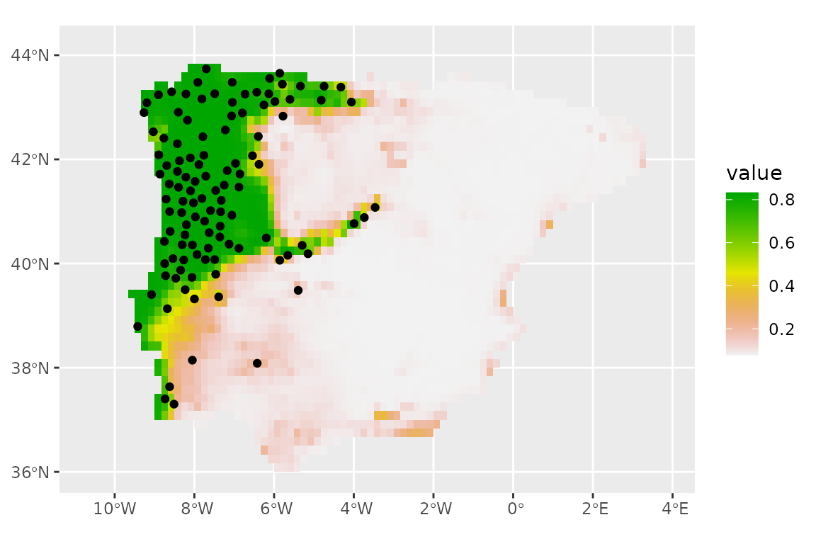
Let us now predict the presence of the lizard in the Iberian
Peninsula using the ensemble. Note that, for
predict_raster() to work, the name and levels for a
categorical variable need to match with those used when training the
models (i.e. in the recipe with step_dummy()):
climate_present <- terra::readRDS(
  system.file("extdata/lacerta_climate_present_10m.rds",
    package = "tidysdm"
  )
)

# project climate layers
iberia_proj4 <- paste0(
  "+proj=aea +lon_0=-4.0 +lat_1=36.8 +lat_2=42.6 ",
  "+lat_0=39.7 +datum=WGS84 +units=m +no_defs"
)
climate_present <- terra::project(climate_present, y = iberia_proj4)

# first we add a topography variable to the climate data
climate_present$topography <- climate_present$altitude
climate_present$topography <- terra::classify(climate_present$topography,
  rcl = c(-Inf, 200, 800, Inf),
  include.lowest = TRUE,
  brackets = TRUE
)
library(terra)
#> terra 1.9.11
#>
#> Attaching package: 'terra'
#> The following object is masked from 'package:tidyr':
#>
#>     extract
#> The following object is masked from 'package:dials':
#>
#>     buffer
#> The following object is masked from 'package:scales':
#>
#>     rescale
levels(climate_present$topography) <-
  data.frame(ID = c(0, 1, 2), topography = c("plains", "hills", "mountains"))

# now we can predict
predict_factor <- predict_raster(lacerta_ensemble, climate_present)

# and plot
ggplot() +
  geom_spatraster(data = predict_factor, aes(fill = mean)) +
  scale_fill_terrain_c() +
  geom_sf(data = lacerta_thin %>% filter(class == "presence"))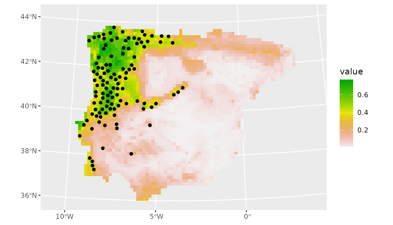
Exploring models with DALEX
An issue with machine learning algorithms is that it is not easy to
understand the role of different variables in giving the final
prediction. A number of packages have been created to explore and
explain the behaviour of ML algorithms, such as those used in
tidysdm. In the tidysdm
overview article, we illustrated how to use recipes to
create profiles.
Here we demonstrate how to use DALEX, an excellent
package that has methods to deal with tidymodels.
tidysdm contains additional functions that allow us to use
the DALEX functions directly on tidysdm ensembles.
We will use a simple ensemble that we built in the overview vignette.
library(tidysdm)
lacerta_ensemble
#> A simple_ensemble of models
#>
#> Members:
#> • default_glm
#> • default_rf
#> • default_gbm
#> • default_maxent
#>
#> Available metrics:
#> • boyce_cont
#> • roc_auc
#> • tss_max
#>
#> Metric used to tune workflows:
#> • boyce_cont
The first step in DALEX is to create an explainer object, which can
then be queried by different functions in the package, to turn the
explainer into an explanation (following the DALEX lingo). As a first
step, we use the custom function explain_tidysdm to
generate our explainer:
explainer_lacerta_ens <- explain_tidysdm(lacerta_ensemble)
#> Preparation of a new explainer is initiated
#>   -> model label       :  data.frame  (  default  )
#>   -> data              :  448  rows  4  cols
#>   -> data              :  tibble converted into a data.frame
#>   -> target variable   :  448  values
#>   -> predict function  :  predict_function
#>   -> predicted values  :  Predict function column set to:  1 (  OK  )
#>   -> model_info        :  package tidysdm , ver. 1.0.4.9002 , task classification (  default  )
#>   -> model_info        :  type set to  classification
#>   -> predicted values  :  numerical, min =  0.02117606 , mean =  0.2977721 , max =  0.8709933
#>   -> residual function :  difference between y and yhat (  default  )
#>   -> residuals         :  numerical, min =  0.1290067 , mean =  1.452228 , max =  1.978824
#>   A new explainer has been created!
Now that we have our explainer, we can explore variable importance for the ensemble:
library(DALEX)
#> Welcome to DALEX (version: 2.5.3).
#> Find examples and detailed introduction at: http://ema.drwhy.ai/
#> Additional features will be available after installation of: ggpubr.
#> Use 'install_dependencies()' to get all suggested dependencies
#>
#> Attaching package: 'DALEX'
#> The following object is masked from 'package:dplyr':
#>
#>     explain
vip_ensemble <- model_parts(explainer = explainer_lacerta_ens)
plot(vip_ensemble)
#> Warning: Using `size` aesthetic for lines was deprecated in ggplot2 3.4.0.
#> ℹ Please use `linewidth` instead.
#> ℹ The deprecated feature was likely used in the ingredients package.
#>   Please report the issue at
#>   <https://github.com/ModelOriented/ingredients/issues>.
#> This warning is displayed once per session.
#> Call `lifecycle::last_lifecycle_warnings()` to see where this warning was
#> generated.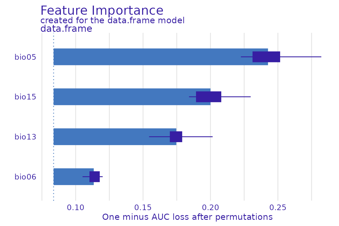
Or generate partial dependency plots for a given variable (e.g. bio05):
pdp_bio05 <- model_profile(explainer_lacerta_ens, N = 500, variables = "bio05")
plot(pdp_bio05)
There are many other functions in DALEX that can be applied to the explainer to further explore the behaviour of the model; see several tutorials on https://modeloriented.github.io/DALEX/ for more details.
It is also possible to explore the individual models that make up the ensemble:
explainer_list <- explain_tidysdm(tidysdm::lacerta_ensemble, by_workflow = TRUE)
#> Warning: Unknown or uninitialised column: `pre`.
#> Preparation of a new explainer is initiated
#>   -> model label       :  default_glm
#>   -> data              :  448  rows  4  cols
#>   -> data              :  tibble converted into a data.frame
#>   -> target variable   :  448  values
#>   -> predict function  :  yhat.workflow  will be used (  default  )
#>   -> predicted values  :  Predict function column set to:  1 (  OK  )
#>   -> model_info        :  package tidymodels , ver. 1.4.1 , task classification (  default  )
#>   -> model_info        :  type set to  classification
#>   -> predicted values  :  numerical, min =  0.01618118 , mean =  0.25 , max =  0.7445644
#>   -> residual function :  difference between y and yhat (  default  )
#>   -> residuals         :  numerical, min =  0.3032477 , mean =  1.5 , max =  1.983819
#>   A new explainer has been created!
#> Warning: Unknown or uninitialised column: `pre`.
#> Preparation of a new explainer is initiated
#>   -> model label       :  default_rf
#>   -> data              :  448  rows  4  cols
#>   -> data              :  tibble converted into a data.frame
#>   -> target variable   :  448  values
#>   -> predict function  :  yhat.workflow  will be used (  default  )
#>   -> predicted values  :  Predict function column set to:  1 (  OK  )
#>   -> model_info        :  package tidymodels , ver. 1.4.1 , task classification (  default  )
#>   -> model_info        :  type set to  classification
#>   -> predicted values  :  numerical, min =  0 , mean =  0.2506163 , max =  0.9258611
#>   -> residual function :  difference between y and yhat (  default  )
#>   -> residuals         :  numerical, min =  0.07413889 , mean =  1.499384 , max =  2
#>   A new explainer has been created!
#> Warning: Unknown or uninitialised column: `pre`.
#> Preparation of a new explainer is initiated
#>   -> model label       :  default_gbm
#>   -> data              :  448  rows  4  cols
#>   -> data              :  tibble converted into a data.frame
#>   -> target variable   :  448  values
#>   -> predict function  :  yhat.workflow  will be used (  default  )
#>   -> predicted values  :  Predict function column set to:  1 (  OK  )
#>   -> model_info        :  package tidymodels , ver. 1.4.1 , task classification (  default  )
#>   -> model_info        :  type set to  classification
#>   -> predicted values  :  numerical, min =  0.0002722652 , mean =  0.2500301 , max =  0.9969552
#>   -> residual function :  difference between y and yhat (  default  )
#>   -> residuals         :  numerical, min =  0.003044844 , mean =  1.49997 , max =  1.999728
#>   A new explainer has been created!
#> Warning: Unknown or uninitialised column: `pre`.
#> Preparation of a new explainer is initiated
#>   -> model label       :  default_maxent
#>   -> data              :  448  rows  4  cols
#>   -> data              :  tibble converted into a data.frame
#>   -> target variable   :  448  values
#>   -> predict function  :  yhat.workflow  will be used (  default  )
#>   -> predicted values  :  Predict function column set to:  1 (  OK  )
#>   -> model_info        :  package tidymodels , ver. 1.4.1 , task classification (  default  )
#>   -> model_info        :  type set to  classification
#>   -> predicted values  :  numerical, min =  0.06587215 , mean =  0.4404422 , max =  0.9522016
#>   -> residual function :  difference between y and yhat (  default  )
#>   -> residuals         :  numerical, min =  0.07163309 , mean =  1.309558 , max =  1.934128
#>   A new explainer has been created!
The resulting list can be then used to build lists of explanations, which can then be plotted.
profile_list <- lapply(explainer_list, model_profile,
  N = 500,
  variables = "bio05"
)
plot(profile_list)
#> Warning: `aes_string()` was deprecated in ggplot2 3.0.0.
#> ℹ Please use tidy evaluation idioms with `aes()`.
#> ℹ See also `vignette("ggplot2-in-packages")` for more information.
#> ℹ The deprecated feature was likely used in the ingredients package.
#>   Please report the issue at
#>   <https://github.com/ModelOriented/ingredients/issues>.
#> This warning is displayed once per session.
#> Call `lifecycle::last_lifecycle_warnings()` to see where this warning was
#> generated.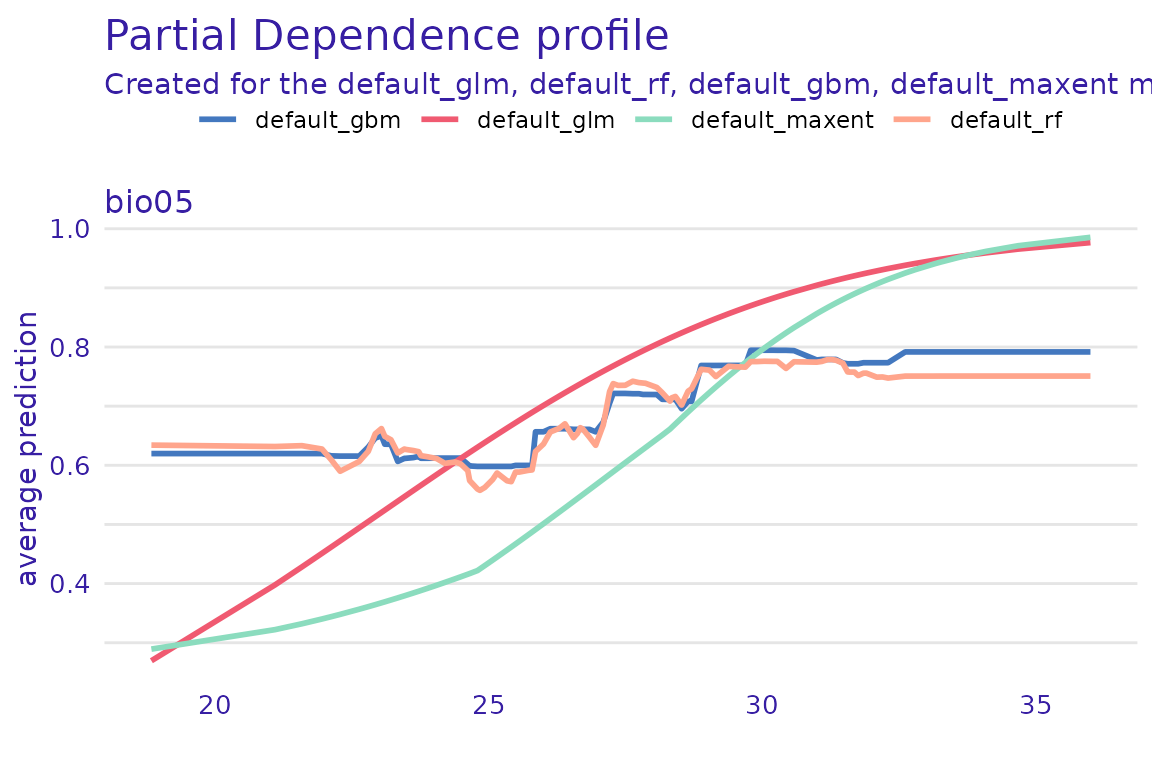
Different recipes for certain models
Some model types (e.g. GLMs and SVMs) can be sensitive to multicollinearity among predictors, while others (notably random forests) are generally more robust to correlated inputs. In this section, we create two separate recipes: one that keeps all predictors, and another that retains only a reduced set of weakly correlated variables.
Load the data:
library(tidysdm)
library(sf)
#> Linking to GEOS 3.12.1, GDAL 3.8.4, PROJ 9.4.0; sf_use_s2() is TRUE
lacerta_thin <- readRDS(system.file("extdata/lacerta_thin_all_vars.rds",
  package = "tidysdm"
))
We then create two recipes: one that keeps all variables, and another that removes highly correlated ones.
lacerta_rec_all <- recipe(lacerta_thin, formula = class ~ .)
lacerta_rec_uncor <- lacerta_rec_all %>%
  step_rm(all_of(c(
    "bio01", "bio02", "bio03", "bio04", "bio07", "bio08",
    "bio09", "bio10", "bio11", "bio12", "bio14", "bio16",
    "bio17", "bio18", "bio19", "altitude"
  )))

lacerta_rec_uncor
#>
#> ── Recipe ──────────────────────────────────────────────────────────────────────
#>
#> ── Inputs
#> Number of variables by role
#> outcome:    1
#> predictor: 20
#> coords:     2
#>
#> ── Operations
#> • Variables removed: all_of(c("bio01", "bio02", "bio03", "bio04", "bio07",
#>   "bio08", "bio09", "bio10", "bio11", "bio12", "bio14", "bio16", "bio17",
#>   "bio18", "bio19", "altitude"))
And now use these two recipes in a workflowset (we will
keep it small for computational time), selecting the appropriate recipe
for each model. We will include a model (polynomial support vector
machines, or SVM) which does not have a wrapper in tidysdm
for creating a model specification. However, we can use a standard model
spec from parsnip:
lacerta_models <-
  # create the workflow_set
  workflow_set(
    preproc = list(
      uncor = lacerta_rec_uncor, # recipe for the glm
      all = lacerta_rec_all, # recipe for the random forest
      uncor = lacerta_rec_uncor # recipe for svm
    ),
    models = list(
      # the standard glm specs
      glm = sdm_spec_glm(),
      # rf specs with tuning
      rf = sdm_spec_rf(),
      # svm specs with tuning
      svm = parsnip::svm_poly(
        cost = tune::tune(),
        degree = tune::tune()
      ) %>%
        parsnip::set_engine("kernlab") %>%
        parsnip::set_mode("classification")
    ),
    # make all combinations of preproc and models,
    cross = FALSE
  ) %>%
  # tweak controls to store information needed later to create the ensemble
  # note that we use the bayes version as we will use a Bayes search (see later)
  option_add(control = stacks::control_stack_bayes())
#> Registered S3 method overwritten by 'butcher':
#>   method                 from
#>   as.character.dev_topic generics
We can now use the block CV folds to tune and assess the models. Note
that there are multiple tuning approaches, besides the standard grid
method. Here we will use tune_bayes from the
tune package (see its help page to see how a Gaussian
Process model is used to choose parameter combinations).
This tuning method (as opposed to use a standard grid) does not allow
for hyper-parameters with unknown limits, but mtry for
random forest is undefined as its upper range depends on the number of
variables in the dataset. So, before tuning, we need to finalise
mtry by informing the set dials with the actual data:
set.seed(100)
# create the CV folds
lacerta_cv <- spatial_block_cv(lacerta_thin, v = 3)

# extract and finalize the rf parameters
rf_param <- lacerta_models %>%
  # extract the rf workflow
  extract_workflow("all_rf") %>%
  # extract its parameters dials (used to tune)
  extract_parameter_set_dials() %>%
  # give it the predictors to finalize mtry
  finalize(x = st_drop_geometry(lacerta_thin) %>% select(-class))

# now update the workflowset with the new parameter info
lacerta_models <- lacerta_models %>%
  option_add(param_info = rf_param, id = "all_rf")
And now we can tune the models:
set.seed(1234567)
lacerta_models <-
  lacerta_models %>%
  workflow_map("tune_bayes",
    resamples = lacerta_cv, initial = 8,
    metrics = sdm_metric_set(), verbose = TRUE
  )
#> Warning: Using `all_of()` outside of a selecting function was deprecated in tidyselect
#> 1.2.0.
#> ℹ See details at
#>   <https://tidyselect.r-lib.org/reference/faq-selection-context.html>
#> This warning is displayed once per session.
#> Call `lifecycle::last_lifecycle_warnings()` to see where this warning was
#> generated.
#> i  No tuning parameters. `fit_resamples()` will be attempted
#> i 1 of 3 resampling: uncor_glm
#> ✔ 1 of 3 resampling: uncor_glm (352ms)
#> i 2 of 3 tuning:     all_rf
#> ! No improvement for 10 iterations; returning current results.
#> ✔ 2 of 3 tuning:     all_rf (17.3s)
#> i 3 of 3 tuning:     uncor_svm
#> maximum number of iterations reached 0.003456553 -0.003390584maximum number of iterations reached 0.004873408 -0.004689518maximum number of iterations reached 2.43803e-05 -2.435951e-05maximum number of iterations reached 0.003562052 -0.003477793maximum number of iterations reached 0.0002060528 -0.0002059063
#> ✔ 3 of 3 tuning:     uncor_svm (21.5s)
We can have a look at the performance of our models with:
autoplot(lacerta_models)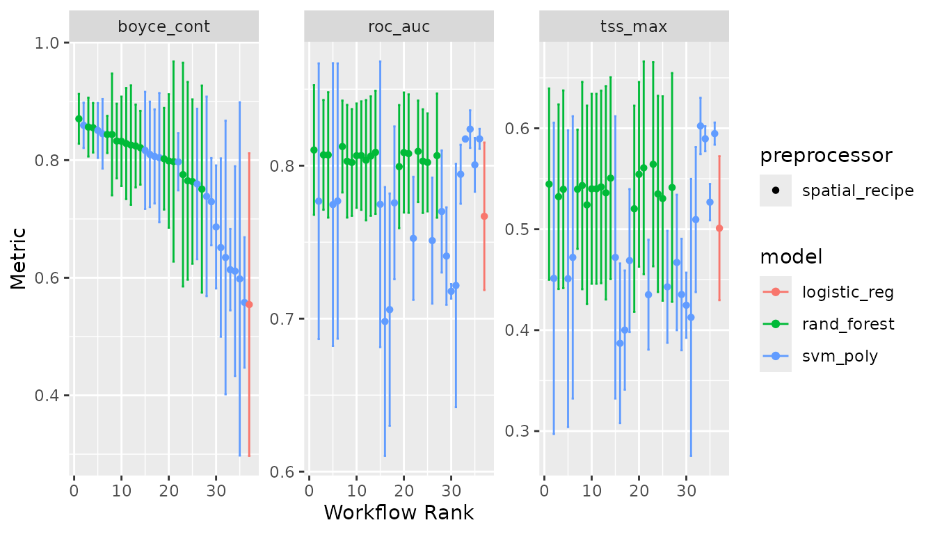
The initial split
The standard tidymodels workflow begins by splitting the
data into a training set (used to fit and tune models)
and an independent testing set (held out for final
evaluation). This step is essential for getting an honest estimate of
predictive performance of any SDM, yet it has often been omitted in
traditional SDM practice, where model assessment has instead relied
primarily on (spatial) cross-validation. This is largely for historical
reasons: SDM datasets were frequently small, and holding data back for
testing felt too costly.
In this section, we demonstrate a robust approach by holding out 20% of the data (1/5) for testing and using the remaining 80% for training. While we strongly recommend this approach whenever the data allow, we acknowledge that it can be data-hungry and may not always be feasible for smaller datasets. We therefore recommend exploring multiple random seeds for the initial split to assess the sensitivity of results to a particular partition, and to avoid splitting the data when results are highly sensitive and unstable.
We start by loading a set of presences and absences and their
associated climate, analogous to the one that we generated in the tidysdm
overview article:
library(tidysdm)
library(sf)
library(tidyterra)
lacerta_thin <- readRDS(system.file("extdata/lacerta_thin_all_vars.rds",
  package = "tidysdm"
))
We then use spatial_initial_split to do the split, using
a spatial_block_cv scheme to partition the data:
set.seed(1005)
lacerta_initial <- spatial_initial_split(lacerta_thin,
  prop = 1 / 5, spatial_block_cv
)
autoplot(lacerta_initial)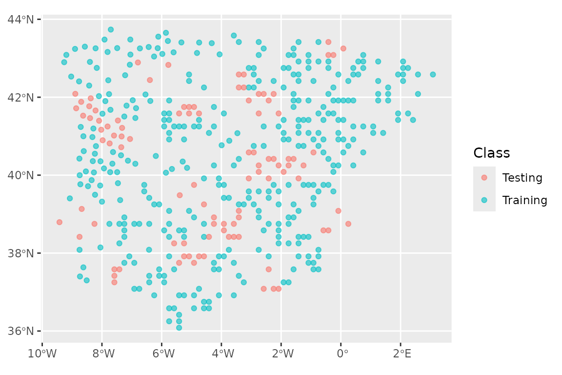
And check the balance of presences vs pseudoabsences:
check_splits_balance(lacerta_initial, class)
#> # A tibble: 1 × 4
#>   presence_test background_test presence_train background_train
#>           <int>           <int>          <int>            <int>
#> 1            86             263             26               73
And confirm that we have the data correctly formatted with:
lacerta_thin %>% check_sdm_presence(class)
#> [1] TRUE
We can now extract the training set from our
lacerta_initial split, and sample folds to set up cross
validation (note that we set the cellsize and
offset based on the full dataset,
lacerta_thin; this allows us to use the same grid we used
for the initial_split). In this example, we also have to
add a very small number to the offset to avoid an error in the
spatial_block_cv function arising from some points falling
on the boundary of the grid cells). This is often not necessary, so only
introduce this if you encounter an error.
set.seed(1005)
lacerta_training <- training(lacerta_initial)
lacerta_cv <- spatial_block_cv(lacerta_training,
  v = 5,
  cellsize = grid_cellsize(lacerta_thin),
  offset = grid_offset(lacerta_thin) + 0.00001
)
autoplot(lacerta_cv)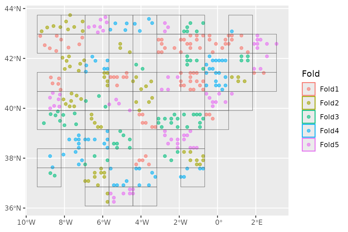
And check the balance in the dataset:
check_splits_balance(lacerta_cv, class)
#> # A tibble: 5 × 4
#>   presence_assessment background_assessment presence_analysis
#>                 <int>                 <int>             <int>
#> 1                  69                   228                17
#> 2                  67                   222                19
#> 3                  62                   191                24
#> 4                  71                   216                15
#> 5                  75                   197                11
#> # ℹ 1 more variable: background_analysis <int>
Next, we need to set up a recipe to define how to handle
our dataset.
lacerta_rec <- recipe(lacerta_training, formula = class ~ .)
lacerta_rec
#>
#> ── Recipe ──────────────────────────────────────────────────────────────────────
#>
#> ── Inputs
#> Number of variables by role
#> outcome:    1
#> predictor: 20
#> coords:     2
Same as in the tidysdm
overview article we can now build a workflow_set of
different models:
lacerta_models <-
  # create the workflow_set
  workflow_set(
    preproc = list(default = lacerta_rec),
    models = list(
      # the standard glm specs
      glm = sdm_spec_glm(),
      # rf specs with tuning
      rf = sdm_spec_rf(),
      # boosted tree model (gbm) specs with tuning
      gbm = sdm_spec_boost_tree(),
      # maxent specs with tuning
      maxent = sdm_spec_maxent()
    ),
    # make all combinations of preproc and models,
    cross = TRUE
  ) %>%
  # tweak controls to store information needed later to create the ensemble
  option_add(control = control_ensemble_grid())
And use the block CV folds to tune and assess the models:
set.seed(1234567)
lacerta_models <-
  lacerta_models %>%
  workflow_map("tune_grid",
    resamples = lacerta_cv, grid = 3,
    metrics = sdm_metric_set(), verbose = TRUE
  )
#> i  No tuning parameters. `fit_resamples()` will be attempted
#> i 1 of 4 resampling: default_glm
#> → A | warning: glm.fit: fitted probabilities numerically 0 or 1 occurred
#> There were issues with some computations   A: x1
#> There were issues with some computations   A: x2
#>
#> ✔ 1 of 4 resampling: default_glm (564ms)
#> i 2 of 4 tuning:     default_rf
#> i Creating pre-processing data to finalize 1 unknown parameter: "mtry"
#> ✔ 2 of 4 tuning:     default_rf (3.7s)
#> i 3 of 4 tuning:     default_gbm
#> i Creating pre-processing data to finalize 1 unknown parameter: "mtry"
#> → A | warning: `early_stop` was reduced to 0.
#> There were issues with some computations   A: x1
#> There were issues with some computations   A: x3
#> There were issues with some computations   A: x4
#> There were issues with some computations   A: x5
#>
#> ✔ 3 of 4 tuning:     default_gbm (11s)
#> i 4 of 4 tuning:     default_maxent
#> ✔ 4 of 4 tuning:     default_maxent (2.4s)

autoplot(lacerta_models)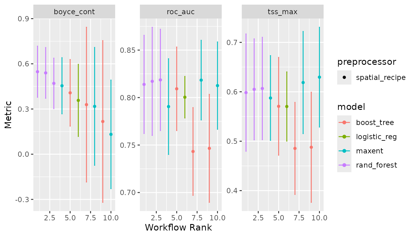
And create an ensemble, selecting the best set of parameters for each model using Boyce continuous index as our metric:
lacerta_ensemble <- simple_ensemble() %>%
  add_member(lacerta_models, metric = "boyce_cont")

autoplot(lacerta_ensemble)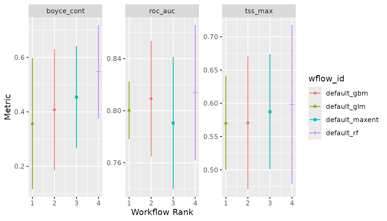
We can now use the ensemble to make predictions about the testing data:
lacerta_testing <- testing(lacerta_initial)

lacerta_test_pred <-
  lacerta_testing %>%
  bind_cols(predict(lacerta_ensemble, ., type = "prob"))
And look at the goodness of fit:
sdm_metric_set()(data = lacerta_test_pred, truth = class, mean)
#> # A tibble: 3 × 3
#>   .metric    .estimator .estimate
#>   <chr>      <chr>          <dbl>
#> 1 boyce_cont binary         0.718
#> 2 roc_auc    binary         0.784
#> 3 tss_max    binary         0.485
We can now make predictions with this ensemble using the best models.
# load climate data
climate_present <- terra::readRDS(
  system.file("extdata/lacerta_climate_present_10m.rds",
    package = "tidysdm"
  )
)

# project climate layers
iberia_proj4 <- paste0(
  "+proj=aea +lon_0=-4.0 +lat_1=36.8 +lat_2=42.6 ",
  "+lat_0=39.7 +datum=WGS84 +units=m +no_defs"
)
climate_present <- terra::project(climate_present, y = iberia_proj4)

# predict using only the best models
prediction_present_boyce <- predict_raster(lacerta_ensemble, climate_present,
  metric_thresh = c("boyce_cont", 0.5),
  fun = "median"
)

# plot
ggplot() +
  geom_spatraster(data = prediction_present_boyce, aes(fill = median)) +
  scale_fill_terrain_c() +
  geom_sf(data = lacerta_thin %>% filter(class == "presence"))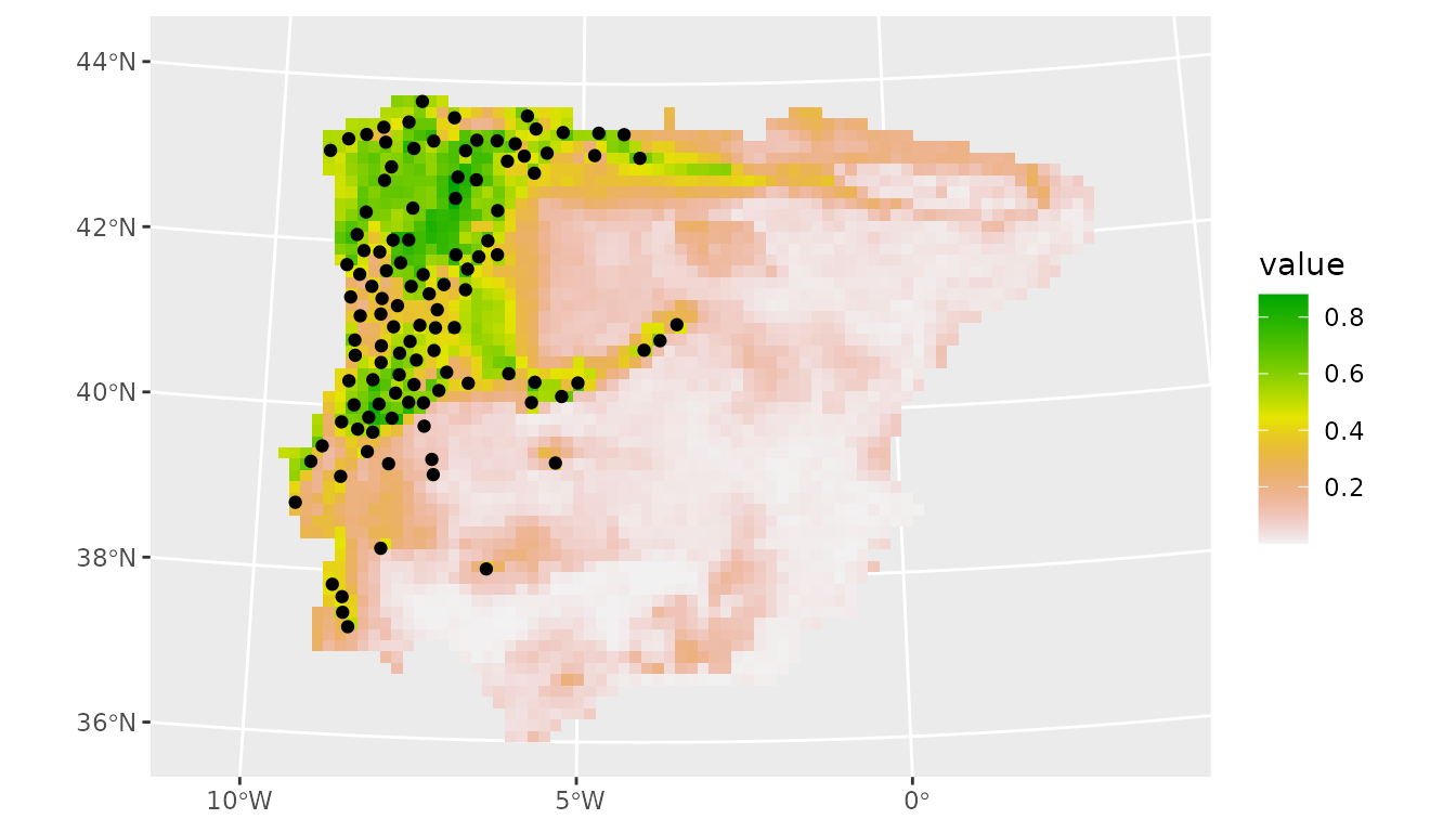
Stack ensembles
Now that we have an explicit training/testing split (see the previous section section), we can go beyond a
simple ensemble that keeps only the single best configuration of each
model type and averages their predictions. Instead, we can build a stack
ensemble using the stacks package. Stacking fits a
meta-learner that learns how to optimally weight predictions from
multiple candidate models, including multiple tuned versions of the same
algorithm with different hyper-parameters, so that the final ensemble
can exploit complementary strengths across model configurations.
An explicit testing split is not strictly required for stacking, since model performance can be estimated using cross-validation. However, an independent test set is recommended whenever an unbiased estimate of the final model’s predictive performance is required. This is particularly important for stacked ensembles, which can be prone to overfitting.
library(stacks)
set.seed(1005)
lacerta_stack <-
  # initialize the stack
  stacks() %>%
  # add candidate members
  add_candidates(lacerta_models) %>%
  # determine how to combine their predictions
  blend_predictions(
    metric = sdm_metric_set() # use our SDM metrics for calculating stacking
    # coefficients
  ) %>%
  # fit candidates with non-zero weights (i.e. non-zero stacking coefficients)
  fit_members()
#> Warning: The inputted `candidates` argument `default_glm` generated notes during
#> tuning/resampling. Model stacking may fail due to these issues; see
#> `collect_notes()` (`?tune::collect_notes()`) if so.
#> Warning: The inputted `candidates` argument `default_gbm` generated notes during
#> tuning/resampling. Model stacking may fail due to these issues; see
#> `collect_notes()` (`?tune::collect_notes()`) if so.

autoplot(lacerta_stack, type = "weights")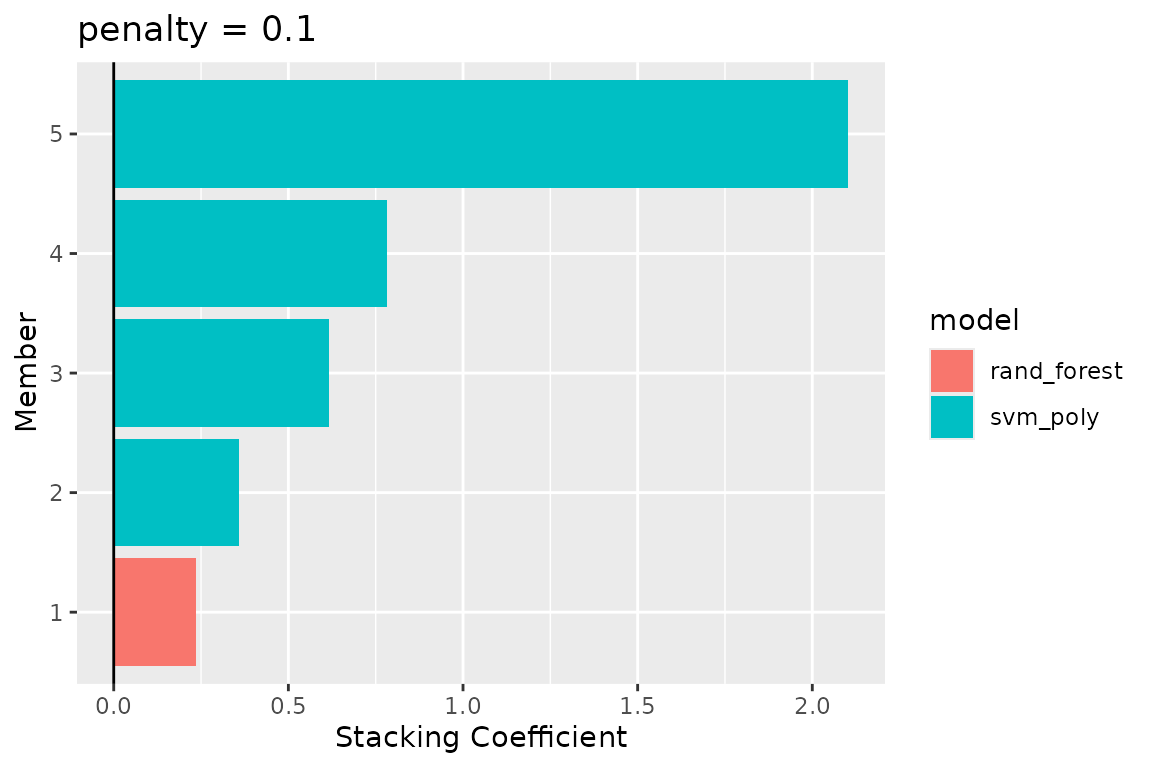
In this example, one random forest variant and one SVM variant were selected (though more can be, depending on tuning and the data). The stacking coefficients indicate how much weight each selected model contributes to the final ensemble prediction. We can now use the ensemble to make predictions about the testing data:
lacerta_testing <- testing(lacerta_initial)

lacerta_test_pred <-
  lacerta_testing %>%
  bind_cols(predict(lacerta_stack, ., type = "prob"))
And look at the goodness of fit using some commonly used sdm metrics.
Note that sdm_metric_set is first invoked to generate a
function (with empty ()) that is then used on the data.
sdm_metric_set()(data = lacerta_test_pred, truth = class, .pred_presence)
#> # A tibble: 3 × 3
#>   .metric    .estimator .estimate
#>   <chr>      <chr>          <dbl>
#> 1 boyce_cont binary         0.464
#> 2 roc_auc    binary         0.823
#> 3 tss_max    binary         0.600
We can now make predictions with this stacked ensemble. We start by extracting the climate for the variables of interest:
climate_present <- terra::readRDS(
  system.file("extdata/lacerta_climate_present_10m.rds",
    package = "tidysdm"
  )
)

# project climate layers
iberia_proj4 <- paste0(
  "+proj=aea +lon_0=-4.0 +lat_1=36.8 +lat_2=42.6",
  " +lat_0=39.7 +datum=WGS84 +units=m +no_defs"
)
climate_present <- terra::project(climate_present, y = iberia_proj4)
And predict the presence of the lizard using the stacked ensemble:
prediction_present <- predict_raster(lacerta_stack, climate_present,
  type = "prob"
)
library(tidyterra)
ggplot() +
  geom_spatraster(data = prediction_present, aes(fill = .pred_presence)) +
  scale_fill_terrain_c() +
  # plot presences used in the model
  geom_sf(data = lacerta_thin %>% filter(class == "presence"))