Human genome diversity panel - georeferenced data

The datasets hgdp and hgdpPlus provides genetic diversity several human populations worldwide. Both datasets are gData objects, interfaced with the gGraph object worldgraph.40k.

Format

hgdp is a gGraph object with the following data: %

@nodes.attr$habitat

habitat corresponding to each % vertice; currently 'land' or 'sea'.

%

@meta$color

a matrix assigning a color for plotting % vertices (second column) to different values of habitat (first % column).

%

Details

hgdp describes 52 populations from the original Human Genome Diversity Panel.

hgdpPlus describes hgdp populations plus 24 native American populations.

References

Authors Journal, YEAR, nb: pp-pp.

Examples

## check object
hgdp
#> 
#> === gData object ===
#> 
#> @coords: spatial coordinates of 52 nodes
#>   lon lat
#> 1  -3  59
#> 2  39  44
#> 3  40  61
#> ...
#> 
#> @nodes.id: nodes identifiers
#>   28179   11012   22532 
#> "26898" "11652" "22532" 
#> ...
#> 
#> @data: 52 data
#>   Population Region Label  n Latitude Longitude Genetic.Div
#> 1   Orcadian EUROPE     1 15       59        -3   0.7258820
#> 2     Adygei EUROPE     2 17       44        39   0.7297802
#> 3    Russian EUROPE     3 25       61        40   0.7319749
#> ...
#> 
#> Associated gGraph: worldgraph.40k 

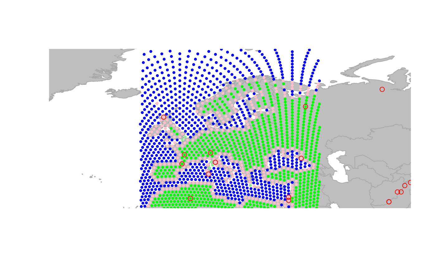
## plotting the object
plot(hgdp)



## results from Handley et al.
if (FALSE) {
## Addis Ababa
addis <- list(lon = 38.74, lat = 9.03)
addis <- closestNode(worldgraph.40k, addis) # this takes a while

## shortest path from Addis Ababa
myPath <- dijkstraFrom(hgdp, addis)

## plot results
plot(worldgraph.40k, col = 0)
points(hgdp)
points(worldgraph.40k[addis], psize = 3, pch = "x", col = "black")
plot(myPath)

## correlations distance/genetic div.
geo.dist <- sapply(myPath[-length(myPath)], function(e) e$length)
gen.div <- getData(hgdp)[, "Genetic.Div"]
plot(gen.div ~ geo.dist)
lm1 <- lm(gen.div ~ geo.dist)
abline(lm1, col = "blue") # this regression is wrong
summary(lm1)
}