Tidy data in population genetics
The fundamental tenet of tidy data that is that each observation should have its own row and each variable its own column, such that each value has its own cell. Applying this logic to population genetic data means that each individual should have its own row, with individual metadata (such as its population, sex, phenotype, etc) as the variables. Genotypes for each locus can also be thought of as variables, however, due to the large number of loci and the restricted values that each genotype can take, it would be very inefficient to store them as individual standard columns.
In tidypopgen, we represent data as a
gen_tbl, a subclass of tibble which has two
compulsory columns: id of the individual (as a
character, which must be unique for each individual), and
genotypes (stored in a compressed format as a File-Backed
Matrix). The genotypes column stores a vector of the row
indices of the matrix for each individual and, when printed, shows the
first two genotypes for the individual.
The real data reside on disk, and an attribute fbm of
the genotype column contains all the information to access
it. There is also an additional attribute, loci which
provides all the information about the loci, including the column
indices that represent each locus in the FBM.
The vector of row indices and the table of loci can be subsetted and
reordered without changing the data on disk; thus, any operation on the
gen_tibble is fast as it shapes the indices of the genotype
matrix rather than the matrix itself.
This is illustrated in the diagram below. Here, we can see the gen_tibble object, the loci table, and the File-Backed Matrix. In the File-Backed Matrix, each row is an individual and each column is a locus. When a function operates on a subset of individuals or loci, the indices of the subset are used to access the relevant rows or columns in the File-Backed Matrix, without needing to load the entire matrix into memory. This makes operations efficient and scalable to large datasets.
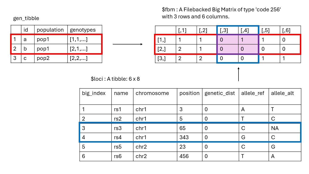
The loci tibble includes columns big_index
for the index in the File-Backed Matrix (or FBM), name for
the locus name (a character, which must be unique),
chromosome for the chromosome (a factor),
position for the position on the chromosome (an
integer, if known, otherwise set to NA),
genetic_dist for the genetic distance on the chromosome
(numeric, if known, else set to 0), allele_ref
for the the reference allele (a character), and
allele_alt for the alternate allele (a
character, which can be 0 for monomorphic
loci, following the same convention as plink). Additional individual
metadata can be stored as columns in the main gen_tbl,
whilst additional loci information (such as the position in
centimorgans) can be added as columns in the loci attribute
table.
In principle, it is possible to use use multiple ways to compress the
genotypes. tidypopgen currently uses a File-Backed Matrix
object from the package bigsnpr. It is very fast and well
documented, but it is mostly geared towards diploid data.
tidypopgen expands that object to deal with different
levels of ploidy, including multiple ploidy within a single dataset;
however, most functions are currently incompatible with ploidy levels
other than 2 (but they will return a clear error message and avoid
computing anything incorrectly).
The grammar of population genetics
The gen_tibble
Given information about the individuals, their genotypes, and the loci:
library(tidypopgen)
#> Loading required package: dplyr
#>
#> Attaching package: 'dplyr'
#> The following objects are masked from 'package:stats':
#>
#>     filter, lag
#> The following objects are masked from 'package:base':
#>
#>     intersect, setdiff, setequal, union
#> Loading required package: tibble
example_indiv_meta <- data.frame(
  id = c("a", "b", "c", "d", "e"),
  population = c("pop1", "pop1", "pop2", "pop2", "pop2")
)
example_genotypes <- rbind(
  c(1, 1, 0, 1, 1, 0),
  c(2, 0, 0, 0, NA, 0),
  c(1, 2, 0, 0, 1, 1),
  c(0, 2, 0, 1, 2, 1),
  c(1, 1, NA, 2, 1, 0)
)
example_loci <- data.frame(
  name = c("rs1", "rs2", "rs3", "rs4", "x1", "x2"),
  chromosome = c(1, 1, 1, 1, 2, 2),
  position = c(3, 5, 65, 343, 23, 456),
  genetic_dist = c(0, 0, 0, 0, 0, 0),
  allele_ref = c("A", "T", "C", "G", "C", "T"),
  allele_alt = c("T", "C", NA, "C", "G", "A")
)
We can create a simple gen_tibble object (of class
gen_tbl) with:
example_gt <- gen_tibble(example_genotypes,
  indiv_meta = example_indiv_meta,
  loci = example_loci,
  backingfile = tempfile()
)
#>
#> gen_tibble saved to /tmp/RtmpgkDI6l/file28034208f6a.gt
#> using FBM RDS: /tmp/RtmpgkDI6l/file28034208f6a.rds
#> with FBM backing file: /tmp/RtmpgkDI6l/file28034208f6a.bk
#> make sure that you do NOT delete those files!
#> to reload the gen_tibble in another session, use:
#> gt_load('/tmp/RtmpgkDI6l/file28034208f6a.gt')
We are provided information on where the three files underlying the
genotype information are stored. As we don’t want to keep the files, we
used the tmp directory; normally you will want to use your working
directory so that the files will not be cleared by R at the end of the
session. It is important that these files are not deleted or moved, as
gen_tibble stores their paths for future use.
Now let’s have a look at our gen_tibble:
example_gt
#> # A gen_tibble: 6 loci
#> # A tibble:     5 × 3
#>   id    population  genotypes
#>   <chr> <chr>      <vctr_SNP>
#> 1 a     pop1        [1,1,...]
#> 2 b     pop1        [2,0,...]
#> 3 c     pop2        [1,2,...]
#> 4 d     pop2        [0,2,...]
#> 5 e     pop2        [1,1,...]
As discussed above, when this tibble is called, the
genotypes column prints the first two genotypes of the
individual. The genotypes column itself contains the
indices of the individuals in the FBM as values, and the FBM as an
attribute.
To retrieve the rest of the genotypes (which are compressed in the FBM), we use:
example_gt %>% show_genotypes()
#>      [,1] [,2] [,3] [,4] [,5] [,6]
#> [1,]    1    1    0    1    1    0
#> [2,]    2    0    0    0   NA    0
#> [3,]    1    2    0    0    1    1
#> [4,]    0    2    0    1    2    1
#> [5,]    1    1   NA    2    1    0
If we want to extract the information about the loci for which we have genotypes (which are stored as an attribute of that column), we say:
example_gt %>% show_loci()
#> # A tibble: 6 × 7
#>   big_index name  chromosome position genetic_dist allele_ref allele_alt
#>       <int> <chr> <fct>         <dbl>        <dbl> <chr>      <chr>
#> 1         1 rs1   1                 3            0 A          T
#> 2         2 rs2   1                 5            0 T          C
#> 3         3 rs3   1                65            0 C          NA
#> 4         4 rs4   1               343            0 G          C
#> 5         5 x1    2                23            0 C          G
#> 6         6 x2    2               456            0 T          A
Note that, if we are passing a gen_tibble to a function
that works on genotypes, it is generally not necessary to pass the
column genotypes in the call:
example_gt %>% indiv_het_obs()
#> [1] 0.6666667 0.0000000 0.5000000 0.3333333 0.6000000
However, if such a function is used within a dplyr verb
such as mutate, we need to pass the genotype
column to the function:
example_gt %>% mutate(het_obs = indiv_het_obs(.data$genotypes))
#> # A gen_tibble: 6 loci
#> # A tibble:     5 × 4
#>   id    population  genotypes het_obs
#>   <chr> <chr>      <vctr_SNP>   <dbl>
#> 1 a     pop1        [1,1,...]   0.667
#> 2 b     pop1        [2,0,...]   0
#> 3 c     pop2        [1,2,...]   0.5
#> 4 d     pop2        [0,2,...]   0.333
#> 5 e     pop2        [1,1,...]   0.6
Or, more simply:
example_gt %>% mutate(het_obs = indiv_het_obs(genotypes))
#> # A gen_tibble: 6 loci
#> # A tibble:     5 × 4
#>   id    population  genotypes het_obs
#>   <chr> <chr>      <vctr_SNP>   <dbl>
#> 1 a     pop1        [1,1,...]   0.667
#> 2 b     pop1        [2,0,...]   0
#> 3 c     pop2        [1,2,...]   0.5
#> 4 d     pop2        [0,2,...]   0.333
#> 5 e     pop2        [1,1,...]   0.6
Standard dplyr verbs to manipulate the tibble
The individual metadata can then be processed with the usual
tidyverse grammar. So, we can filter individuals by
population with
example_pop2 <- example_gt %>% filter(population == "pop2")
example_pop2
#> # A gen_tibble: 6 loci
#> # A tibble:     3 × 3
#>   id    population  genotypes
#>   <chr> <chr>      <vctr_SNP>
#> 1 c     pop2        [1,2,...]
#> 2 d     pop2        [0,2,...]
#> 3 e     pop2        [1,1,...]
There are a number of functions that compute population genetics quantities for each individual, such as individual observed heterozygosity. We can compute them simply with:
example_gt %>% indiv_het_obs()
#> [1] 0.6666667 0.0000000 0.5000000 0.3333333 0.6000000
Or after filtering:
example_gt %>%
  filter(population == "pop2") %>%
  indiv_het_obs()
#> [1] 0.5000000 0.3333333 0.6000000
We can use mutate to add observed heterozygosity as a
column to our gen_tibble (again, note that functions that
work on genotypes don’t need to be passed any arguments if the tibble is
passed directly to them, but the column genotypes has to be
provided when they are used within dplyr verbs such as
mutate):
example_gt %>% mutate(het_obs = indiv_het_obs(genotypes))
#> # A gen_tibble: 6 loci
#> # A tibble:     5 × 4
#>   id    population  genotypes het_obs
#>   <chr> <chr>      <vctr_SNP>   <dbl>
#> 1 a     pop1        [1,1,...]   0.667
#> 2 b     pop1        [2,0,...]   0
#> 3 c     pop2        [1,2,...]   0.5
#> 4 d     pop2        [0,2,...]   0.333
#> 5 e     pop2        [1,1,...]   0.6
There are a number of functions that estimate quantities at the
individual level, and they are prefixed by
indiv_.
Using verbs on loci
Since the genotypes of the loci are stored as a compressed list in
one column, it is not possible to use standard dplyr verbs
on them. However, tidypopgen provides a number of
specialised verbs, postfixed by _loci, to manipulate
loci.
A key operation on loci is their selection (and removal). The
compressed nature of genotypes imposes some constraints on the possible
grammar. For selection, there are two verbs: select_loci
and select_loci_if. select_loci understands
the concise-minilanguage spoken by standard dplyr::select
that allows to easily refer to variables by their names. However,
select_loci criteria can not be based on the actual
genotypes (e.g. on heterozygosity or missingness). For that, we have to
use select_loci_if, which can operate on the genotypes but
is blind to the names of loci.
Let us start by looking at the loci names in our simple dataset:
loci_names(example_gt)
#> [1] "rs1" "rs2" "rs3" "rs4" "x1"  "x2"
We can see that there are two categories of loci, one starting with “rs” and the other with “x”. If we wanted to select only loci that have an “rs” code, we would use:
example_sub <- example_gt %>% select_loci(starts_with("rs"))
example_sub
#> # A gen_tibble: 4 loci
#> # A tibble:     5 × 3
#>   id    population  genotypes
#>   <chr> <chr>      <vctr_SNP>
#> 1 a     pop1        [1,1,...]
#> 2 b     pop1        [2,0,...]
#> 3 c     pop2        [1,2,...]
#> 4 d     pop2        [0,2,...]
#> 5 e     pop2        [1,1,...]
This gives us a gen_tibble with only 4 loci, as
expected. We can confirm that we have the correct loci with:
loci_names(example_sub)
#> [1] "rs1" "rs2" "rs3" "rs4"
Let us check that this has indeed impacted the individual heterozygosity
example_sub %>% indiv_het_obs()
#> [1] 0.5000000 0.0000000 0.1666667 0.1666667 0.4000000
We can also subset and reorder by passing indices:
example_gt %>%
  select_loci(c(2, 6, 1)) %>%
  show_loci()
#> # A tibble: 3 × 7
#>   big_index name  chromosome position genetic_dist allele_ref allele_alt
#>       <int> <chr> <fct>         <dbl>        <dbl> <chr>      <chr>
#> 1         2 rs2   1                 5            0 T          C
#> 2         6 x2    2               456            0 T          A
#> 3         1 rs1   1                 3            0 A          T
This operation could be helpful when merging datasets that do not fully overlap on their loci (more on that later).
example_gt %>%
  select_loci(c(2, 6, 1)) %>%
  show_genotypes()
#>      [,1] [,2] [,3]
#> [1,]    1    0    1
#> [2,]    0    0    2
#> [3,]    2    1    1
#> [4,]    2    1    0
#> [5,]    1    0    1
The limit of select_loci is that it can not directly
summarise the genotypes. We can do that separately and then feed the
result as a set of indices. For example, we might want to impose a
minimum minor allele frequency. loci_maf() allows us to
inspect the minimum allele frequencies in a gen_tibble:
We can now create a vector of indices of loci with a minimum allele frequency (MAF) larger than 0.2, and use it to select:
sel_indices <- which((example_gt %>% loci_maf()) > 0.2)
example_gt %>%
  select_loci(all_of(sel_indices)) %>%
  show_loci()
#> # A tibble: 4 × 7
#>   big_index name  chromosome position genetic_dist allele_ref allele_alt
#>       <int> <chr> <fct>         <dbl>        <dbl> <chr>      <chr>
#> 1         1 rs1   1                 3            0 A          T
#> 2         2 rs2   1                 5            0 T          C
#> 3         4 rs4   1               343            0 G          C
#> 4         5 x1    2                23            0 C          G
Note that passing a variable directly to select is
deprecated, and so we have to use all_of to wrap it.
select_loci_if allows us to avoid creating a temporary
variable to store indices:
example_gt_sub <- example_gt %>% select_loci_if(loci_maf(genotypes) > 0.2)
example_gt_sub %>% show_genotypes()
#>      [,1] [,2] [,3] [,4]
#> [1,]    1    1    1    1
#> [2,]    2    0    0   NA
#> [3,]    1    2    0    1
#> [4,]    0    2    1    2
#> [5,]    1    1    2    1
Note that, as we need to tidy evaluate loci_maf within
the select_loci_if verb, we need to provide it with the
column that we want to use (even though it has to be
genotypes). Also note that, with
select_loci_if, we cannot reorder the loci.
select_loci_if is very flexible; for example, we could
filter loci with a MAF greater than 0.2 that are also on chromosome
2.
We can use a similar approach to select only alleles on a given chromosome:
example_gt %>%
  select_loci_if(
    loci_chromosomes(genotypes) == 2 &
      loci_maf(genotypes) > 0.2
  ) %>%
  show_loci()
#> # A tibble: 1 × 7
#>   big_index name  chromosome position genetic_dist allele_ref allele_alt
#>       <int> <chr> <fct>         <dbl>        <dbl> <chr>      <chr>
#> 1         5 x1    2                23            0 C          G
Incidentally, loci_maf() is one of several functions
that compute quantities by locus; they can be identified as they start
with loci_.
Grouping individuals in populations
In population genetics, we are generally interested in computing quantities that describe groups of individuals (i.e. populations). Grouping can be used in a number of ways.
As a starting point, we can group by population and get pop sizes:
example_gt %>%
  group_by(population) %>%
  tally()
#> # A tibble: 2 × 2
#>   population     n
#>   <chr>      <int>
#> 1 pop1           2
#> 2 pop2           3
For functions that return one result per individual (such as
indiv_het_obs that we used before), we can use
summarise, which returns a new tibble with one
line per population. For example, we can count the number of individuals
per population, as well as their mean heterozygosity with :
example_gt %>%
  group_by(population) %>%
  summarise(n = n(), mean_het = mean(indiv_het_obs(genotypes)))
#> # A tibble: 2 × 3
#>   population     n mean_het
#>   <chr>      <int>    <dbl>
#> 1 pop1           2    0.333
#> 2 pop2           3    0.478
However, note that this is somewhat inefficient, as computing the pop averages requires multiple access to the data. A more efficient approach is to:
example_gt %>%
  mutate(het_obs = indiv_het_obs(genotypes)) %>%
  group_by(population) %>%
  summarise(n = n(), mean_het = mean(het_obs))
#> # A tibble: 2 × 3
#>   population     n mean_het
#>   <chr>      <int>    <dbl>
#> 1 pop1           2    0.333
#> 2 pop2           3    0.478
In this way, we compute all individual heterozygosities in one go (optimising our file access time), and then generate the population summaries.
When working with loci, you can use reframe to apply
functions across groups. To use reframe correctly, be sure
to select the genotype column within the loci verbs:
example_gt %>%
  group_by(population) %>%
  reframe(loci_hwe = loci_hwe(genotypes))
#> # A tibble: 12 × 2
#>    population loci_hwe
#>    <chr>         <dbl>
#>  1 pop1            0.5
#>  2 pop1            0.5
#>  3 pop1            0.5
#>  4 pop1            0.5
#>  5 pop1            0.5
#>  6 pop1            0.5
#>  7 pop2            0.6
#>  8 pop2            0.5
#>  9 pop2            0.5
#> 10 pop2            0.7
#> 11 pop2            0.6
#> 12 pop2            0.6
Some functions, such as loci_maf(), also have a method
for grouped tibbles that allows an even easier syntax:
example_gt %>%
  group_by(population) %>%
  loci_maf()
#> # A tibble: 12 × 3
#>    loci  group value
#>    <chr> <chr> <dbl>
#>  1 rs1   pop1  0.25
#>  2 rs1   pop2  0.333
#>  3 rs2   pop1  0.25
#>  4 rs2   pop2  0.167
#>  5 rs3   pop1  0
#>  6 rs3   pop2  0
#>  7 rs4   pop1  0.25
#>  8 rs4   pop2  0.5
#>  9 x1    pop1  0.5
#> 10 x1    pop2  0.333
#> 11 x2    pop1  0
#> 12 x2    pop2  0.333
These methods are coded in C++ to be very efficient, and they should
be preferred to the reframe() option. By default, their
outputs will return a tidy tibble, with one row per locus per population
(i.e. the same as we would get with reframe()). However,
using the type argument, it is also possible to return a
list:
example_gt %>%
  group_by(population) %>%
  loci_maf(type = "list")
#> [[1]]
#> [1] 0.25 0.25 0.00 0.25 0.50 0.00
#>
#> [[2]]
#> [1] 0.3333333 0.1666667 0.0000000 0.5000000 0.3333333 0.3333333
Or a matrix:
example_gt %>%
  group_by(population) %>%
  loci_maf(type = "matrix")
#>     pop1      pop2
#> rs1 0.25 0.3333333
#> rs2 0.25 0.1666667
#> rs3 0.00 0.0000000
#> rs4 0.25 0.5000000
#> x1  0.50 0.3333333
#> x2  0.00 0.3333333
Certain metrics and analyses are naturally defined by a grouped tibble as they refer to populations, such as population-specific Fst. For example:
These type of functions are prefixed with pop.
Functions applying to all pairwise and nwise combinations of individuals or populations
The final group of verbs are prefixed by pairwise_ and
nwise_, and they are designed to compute pairwise
statistics between all pairs or combinations of n individuals or
populations (when targeting populations, we start with
pairwise_pop_ and nwise_pop_). For example, to
get the Identity by State for all pairs of individuals, we use:
example_gt %>%
  pairwise_ibs()
#> # A tibble: 10 × 3
#>    item1 item2 value
#>    <chr> <chr> <dbl>
#>  1 a     b     0.7
#>  2 a     c     0.75
#>  3 a     d     0.667
#>  4 a     e     0.9
#>  5 b     c     0.6
#>  6 b     d     0.4
#>  7 b     e     0.5
#>  8 c     d     0.75
#>  9 c     e     0.6
#> 10 d     e     0.5
Reading data
As we saw at the beginning of this vignette, it is possible to create
a gen_tibble with data in data.frames and tibbles. We can
use that function to wrangle small datasets in custom formats, but more
commonly SNP data are stored as PLINK bed files or VCF files.
gen_tibble can directly read both types of files (including
gzipped vcf files), we just need to provide the path to file as the
first argument of gen_tibble; for example, if we want to
read a PLINK bed file, we can simply use:
bed_path_pop_a <- system.file("extdata/pop_a.bed", package = "tidypopgen")
pop_a_gt <- gen_tibble(bed_path_pop_a, backingfile = tempfile("pop_a_"))
#>
#> gen_tibble saved to /tmp/RtmpgkDI6l/pop_a_280328c284bf.gt
#> using FBM RDS: /tmp/RtmpgkDI6l/pop_a_280328c284bf.rds
#> with FBM backing file: /tmp/RtmpgkDI6l/pop_a_280328c284bf.bk
#> make sure that you do NOT delete those files!
#> to reload the gen_tibble in another session, use:
#> gt_load('/tmp/RtmpgkDI6l/pop_a_280328c284bf.gt')
For this vignette, we don’t want to keep files, so we are using again
a temporary path for the backing files, but in normal instances, we can
simply omit the backingfile parameter, and the
.rds and .bk file will be saved with the same
name and path as the original .bed file.
We can also export data into various formats with the family of
functions gt_as_*(). Some functions, such as
gt_as_hierfstat(), gt_as_genind() or
gt_as_genlight() return an object of the appropriate type;
other functions, such as gt_as_plink() or
gt_as_geno_lea() write a file in the appropriate format,
and return the name of that file on completion. For example, to export
to a PLINK .bed file, we simply use:
gt_as_plink(example_gt, file = tempfile("new_bed_"))
#> [1] "/tmp/RtmpgkDI6l/new_bed_2803269d8477.bed"
This will also write a .bim and .fam file and save them together with
the .bed file. Note that, from the main tibble, only id,
population and sex will be preserved in the
.fam file. It is also possible to write .ped and .raw files by
specifying type="ped" or type="raw" in
gt_as_plink() (see the help page for
gt_as_plink() for details).
Merging data
Merging data from different sources is a common problem, especially
in human population genetics where there is a wealth of SNP chips
available. In tidypopgen, merging is enacted with an
rbind operation between gen_tibbles. If the
datasets have the same loci, then the merge is trivial. If not, then it
is necessary to subset to the same loci, and ensure that the data are
coded with the same reference and alternate alleles (or swap if needed).
Additionally, if data come from SNP chips, there is the added
complication that the strand is not always consistent, so it might also
be necessary to flip strand (in that case, ambiguous SNPs have to be
filtered). The rbind method for gen_tibbles
has a number of parameters that allow us to control the behaviour of the
merge.
Let us start by bringing in two sample datasets (note that we use tempfiles to store the data; in real applications, we will usually avoid defining a backingfile and let the function create backing files where the bed file is stored):
bed_path_pop_a <- system.file("extdata/pop_a.bed", package = "tidypopgen")
pop_a_gt <- gen_tibble(bed_path_pop_a, backingfile = tempfile("pop_a_"))
#>
#> gen_tibble saved to /tmp/RtmpgkDI6l/pop_a_280352b2f4cd.gt
#> using FBM RDS: /tmp/RtmpgkDI6l/pop_a_280352b2f4cd.rds
#> with FBM backing file: /tmp/RtmpgkDI6l/pop_a_280352b2f4cd.bk
#> make sure that you do NOT delete those files!
#> to reload the gen_tibble in another session, use:
#> gt_load('/tmp/RtmpgkDI6l/pop_a_280352b2f4cd.gt')
bed_path_pop_b <- system.file("extdata/pop_b.bed", package = "tidypopgen")
pop_b_gt <- gen_tibble(bed_path_pop_b, backingfile = tempfile("pop_b_"))
#>
#> gen_tibble saved to /tmp/RtmpgkDI6l/pop_b_28031f679dac.gt
#> using FBM RDS: /tmp/RtmpgkDI6l/pop_b_28031f679dac.rds
#> with FBM backing file: /tmp/RtmpgkDI6l/pop_b_28031f679dac.bk
#> make sure that you do NOT delete those files!
#> to reload the gen_tibble in another session, use:
#> gt_load('/tmp/RtmpgkDI6l/pop_b_28031f679dac.gt')
And inspect them:
pop_a_gt
#> # A gen_tibble: 16 loci
#> # A tibble:     5 × 4
#>   id    population sex    genotypes
#>   <chr> <chr>      <fct> <vctr_SNP>
#> 1 GRC24 pop_a      male   [0,0,...]
#> 2 GRC25 pop_a      male   [0,0,...]
#> 3 GRC26 pop_a      male   [0,1,...]
#> 4 GRC27 pop_a      male   [0,0,...]
#> 5 GRC28 pop_a      male   [0,0,...]
And the other one:
pop_b_gt
#> # A gen_tibble: 17 loci
#> # A tibble:     3 × 4
#>   id     population sex     genotypes
#>   <chr>  <chr>      <fct>  <vctr_SNP>
#> 1 SL088  pop_b      female  [0,0,...]
#> 2 SL1329 pop_b      female  [1,1,...]
#> 3 SL1108 pop_b      male    [0,1,...]
Here we are using very small datasets, but in real life,
rbind operations are very demanding. Before performing such
an operation, we can run rbind_dry_run:
report <- rbind_dry_run(pop_a_gt, pop_b_gt, flip_strand = TRUE)
#> harmonising loci between two datasets
#> flip_strand =  TRUE  ; remove_ambiguous =  TRUE
#> -----------------------------
#> dataset: reference
#> number of SNPs: 16 reduced to 12
#> ( 2 are ambiguous, of which 2  were removed)
#> -----------------------------
#> dataset: target
#> number of SNPs: 17 reduced to 12
#> ( 5 were flipped to match the reference set)
#> ( 2 are ambiguous, of which 2 were removed)
Note that, by default, rbind will NOT flip strand or
remove ambiguous SNPs (as they are only relevant when merging different
SNP chips), you need to set flip_strand to TRUE.
The report object contains details about why each locus was either
kept or removed, but usually the report is sufficient to make decisions
on whether we want to go ahead. If we are happy with the likely outcome,
we can proceed with the rbind. Note that the data will be
saved to disk. We can either provide a path and prefix, to which ‘.RDS’
and ‘.bk’ will be appended for the R object and associated File-Backed
Matrix; or let the function save the files in the same path as the
original backing file of the first object).
NOTE: In this vignette, we save to the temporary directory, but in real life you want to save in a directory where you will be able to retrieve the file at a later date!!!
# #create merge
merged_gt <- rbind(pop_a_gt, pop_b_gt,
  flip_strand = TRUE,
  backingfile = file.path(tempdir(), "gt_merged")
)
#> harmonising loci between two datasets
#> flip_strand =  TRUE  ; remove_ambiguous =  TRUE
#> -----------------------------
#> dataset: reference
#> number of SNPs: 16 reduced to 12
#> ( 2 are ambiguous, of which 2  were removed)
#> -----------------------------
#> dataset: target
#> number of SNPs: 17 reduced to 12
#> ( 5 were flipped to match the reference set)
#> ( 2 are ambiguous, of which 2 were removed)
#>
#> gen_tibble saved to /tmp/RtmpgkDI6l/gt_merged.gt
#> using FBM RDS: /tmp/RtmpgkDI6l/gt_merged.rds
#> with FBM backing file: /tmp/RtmpgkDI6l/gt_merged.bk
#> make sure that you do NOT delete those files!
#> to reload the gen_tibble in another session, use:
#> gt_load('/tmp/RtmpgkDI6l/gt_merged.gt')
Let’s check the resulting gen_tibble:
merged_gt
#> # A gen_tibble: 12 loci
#> # A tibble:     8 × 4
#>   id     population sex     genotypes
#>   <chr>  <chr>      <fct>  <vctr_SNP>
#> 1 GRC24  pop_a      male    [0,0,...]
#> 2 GRC25  pop_a      male    [0,0,...]
#> 3 GRC26  pop_a      male    [1,1,...]
#> 4 GRC27  pop_a      male    [0,0,...]
#> 5 GRC28  pop_a      male    [0,1,...]
#> 6 SL088  pop_b      female  [0,0,...]
#> 7 SL1329 pop_b      female  [1,1,...]
#> 8 SL1108 pop_b      male    [0,1,...]
We can look at the subsetted loci (note that we used the first population as reference to determine the strand and order of alleles):
merged_gt %>% show_loci()
#> # A tibble: 12 × 7
#>    big_index name       chromosome  position genetic_dist allele_ref allele_alt
#>        <int> <chr>      <fct>          <int>        <dbl> <chr>      <chr>
#>  1         1 rs3094315  1             752566            0 A          G
#>  2         2 rs3131972  1             752721            0 G          A
#>  3         3 rs12124819 1             776546            0 A          G
#>  4         4 rs11240777 1             798959            0 G          A
#>  5         5 rs1110052  1             873558            0 G          T
#>  6         6 rs6657048  1             957640            0 C          T
#>  7         7 rs2488991  1             994391            0 T          G
#>  8         8 rs2862633  2           61974443            0 G          A
#>  9         9 rs28569024 2          139008811            0 T          C
#> 10        10 rs10106770 2          235832763            0 G          A
#> 11        11 rs11942835 3          155913651            0 T          C
#> 12        12 rs5945676  23          51433071            0 T          G
Note that the big_index values have changed compared to
the original files, as we generated a new FBM with the merged data.
By default, rbind using the loci names to match the two
datasets. The option ‘use_position = TRUE’ forces matching by chromosome
and position; note that a common source of problems when merging is the
coding of chromosomes (e.g. a dataset has ‘chromosome1’ and the other
‘chr1’). If using ‘use_position = TRUE’, you should also make sure that
the two datasets were aligned to the same reference genome assembly.
Imputation
Many genetic analysis (e.g. PCA) do not allow missing data. In many
software implementations, missing genotypes are imputed on the fly,
often in a simplistic manner. In tidypopgen, we encourage
taking this step explicitly, before running any analysis.
Let us start with a dataset that has some missing genotypes:
bed_file <- system.file("extdata", "example-missing.bed", package = "bigsnpr")
missing_gt <- gen_tibble(bed_file, backingfile = tempfile("missing_"))
#>
#> gen_tibble saved to /tmp/RtmpgkDI6l/missing_28036eb4b039.gt
#> using FBM RDS: /tmp/RtmpgkDI6l/missing_28036eb4b039.rds
#> with FBM backing file: /tmp/RtmpgkDI6l/missing_28036eb4b039.bk
#> make sure that you do NOT delete those files!
#> to reload the gen_tibble in another session, use:
#> gt_load('/tmp/RtmpgkDI6l/missing_28036eb4b039.gt')
missing_gt
#> # A gen_tibble: 500 loci
#> # A tibble:     200 × 3
#>    id     population  genotypes
#>    <chr>  <chr>      <vctr_SNP>
#>  1 ind_1  fam_1       [0,.,...]
#>  2 ind_2  fam_2       [0,.,...]
#>  3 ind_3  fam_3       [0,0,...]
#>  4 ind_4  fam_4       [.,0,...]
#>  5 ind_5  fam_5       [0,0,...]
#>  6 ind_6  fam_6       [0,0,...]
#>  7 ind_7  fam_7       [0,0,...]
#>  8 ind_8  fam_8       [0,0,...]
#>  9 ind_9  fam_9       [0,0,...]
#> 10 ind_10 fam_10      [0,0,...]
#> # ℹ 190 more rows
We can visualise the amount of missingness with:
missing_gt %>%
  loci_missingness() %>%
  hist()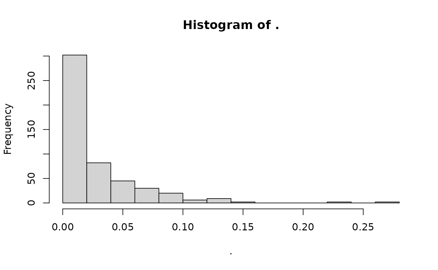
If we attempt to run a PCA on this dataset, we get:
missing_pca <- missing_gt %>% gt_pca_autoSVD()
#> Error:
#> ! You can't have missing values in 'G'.
Note that using gt_pca_autoSVD with a small dataset will likely cause an error, see manual page for details.
It is possible to obviate to this problem by filtering loci with
missing data, but that might lose a lot of loci. The alternative is to
impute the missing the data. tidypopgen provides a wrapper
for fast imputation available in bigsnpr, a simple
imputation (gt_impute_simple) based on the frequency of the
alleles at each locus (by random sampling, or using the mean or mode).
These methods are fine to impute a few missing genotypes, but they
should not be used for any sophisticated imputation (e.g. of low
coverage genomes).
We use the simple approach to fix our dataset:
missing_gt <- gt_impute_simple(missing_gt, method = "mode")We can now check that our dataset has indeed been imputed:
gt_has_imputed(missing_gt)
#> [1] TRUE
However, note that a gen_tibble stores both the raw data
and the imputed data. Even after imputation, the imputed data are not
used by default:
gt_uses_imputed(missing_gt)
#> [1] FALSE
And indeed, if we summarise missingness, we still get:
missing_gt %>%
  loci_missingness() %>%
  hist()
We can manually force a gen_tibble to use the imputed
data:
gt_set_imputed(missing_gt, set = TRUE)
missing_gt %>%
  loci_missingness() %>%
  hist()
However, this is generally not needed, we can keep our
gen_tibble set to use the raw data:
gt_set_imputed(missing_gt, set = FALSE)
missing_gt %>%
  loci_missingness() %>%
  hist()
And let functions that need imputation use it automatically:
missing_pca <- missing_gt %>% gt_pca_partialSVD()
missing_pca
#>  === PCA of gen_tibble object ===
#> Method: [1] "partialSVD"
#>
#> Call ($call):gt_pca_partialSVD(x = .)
#>
#> Eigenvalues ($d):
#>  146.859 106.219 90.352 80.983 69.332 68.427 ...
#>
#> Principal component scores ($u):
#>  matrix with 200 rows (individuals) and 10 columns (axes)
#>
#> Loadings (Principal axes) ($v):
#>  matrix with 500 rows (SNPs) and 10 columns (axes)
Note that, when the function is finished, the gen_tibble
is back to using the raw genotypes:
gt_uses_imputed(missing_gt)
#> [1] FALSE
missing_gt %>%
  loci_missingness() %>%
  hist()
More details about PCA and other analysis is found in the vignette on population genetic analysis.
Saving data and updating backingfiles
We can save a gen_tibble with gt_save().
This command will save a file with extension .gt. We may
want to use gt_save() if we have added any columns of
metadata to our gen_tibble, or if we have subset the
individuals in our gen_tibble, then we can reload the same
object in the next R session.
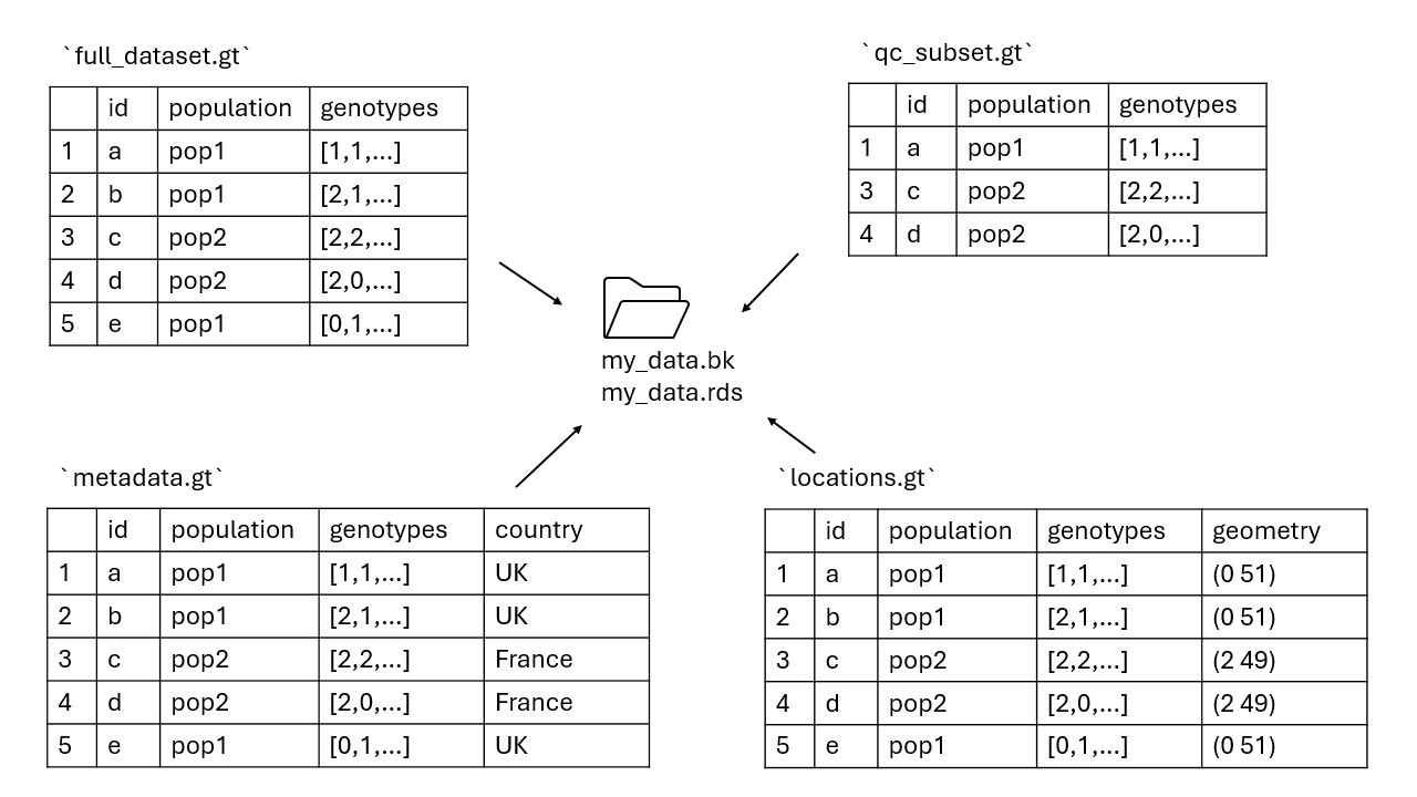
The .gt file works together with the .rds
and .bk files to include all the information stored in the
gen_tibble. However, several gen_tibble
objects can work with the same .rds and .bk
files (for example, if we create different subsets of individuals or
loci).
The .rds and .bk file must share a name,
but the .gt file can be named differently. By default, if
no specific name is given gt_save will use the same pattern
as the .rds and .bk file, and if that pattern
is already in use by another .gt object, a version number
will be appended. You may want to name your .gt files
according to the content of the gen_tibble object (for
example, indicating which individuals and loci are included).
The schematic below illustrates this, where multiple
gen_tibble objects use the same backingfiles.
So, let us save our file:
gt_file_name <- gt_save(example_gt)
#>
#> gen_tibble saved to /tmp/RtmpgkDI6l/file28034208f6a.gt
#> using FBM RDS: /tmp/RtmpgkDI6l/file28034208f6a.rds
#> with FBM backing file: /tmp/RtmpgkDI6l/file28034208f6a.bk
#> make sure that you do NOT delete those files!
#> to reload the gen_tibble in another session, use:
#> gt_load('/tmp/RtmpgkDI6l/file28034208f6a.gt')
gt_file_name
#> [1] "/tmp/RtmpgkDI6l/file28034208f6a.gt"  "/tmp/RtmpgkDI6l/file28034208f6a.rds"
#> [3] "/tmp/RtmpgkDI6l/file28034208f6a.bk"
And if we ever need to retrieve the location of the .bk
and .rds files for a gen_tibble, we can use:
gt_get_file_names(example_gt)
#> [1] "/tmp/RtmpgkDI6l/file28034208f6a.rds" "/tmp/RtmpgkDI6l/file28034208f6a.bk"
In a later session, we could reload the data with:
new_example_gt <- gt_load(gt_file_name[1])
new_example_gt %>% show_genotypes()
#>      [,1] [,2] [,3] [,4] [,5] [,6]
#> [1,]    1    1    0    1    1    0
#> [2,]    2    0    0    0   NA    0
#> [3,]    1    2    0    0    1    1
#> [4,]    0    2    0    1    2    1
#> [5,]    1    1   NA    2    1    0
We can see that our genotypes were recovered correctly.
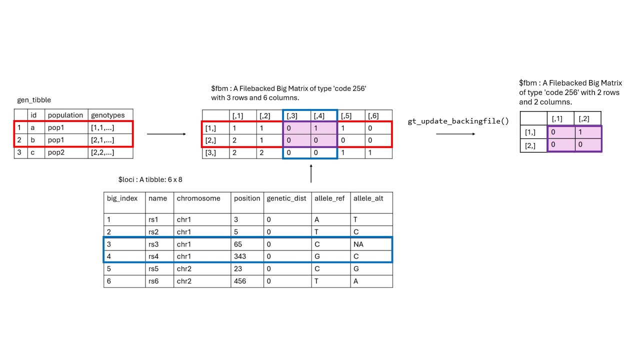
Occasionally, we may need to update the backing files of a
gen_tibble (the .rds and .bk
files), as some functions require that the number of individuals in the
gen_tibble object loaded in the R session matches the
number of individuals in the backing files that are stored on disk. The
schematic below illustrates this.
For example, lets assume we want to impute missing values in our data. In our QC step we may have filtered out some individuals, like so:
But now when we try to impute using the function
gt_impute_simple, we get the following error:
gt_impute_simple(new_example_gt)
#> Error in `gt_impute_simple()`:
#> ! The number of individuals in the gen_tibble does not match the number of rows in the file backing matrix. Before imputing, use gt_update_backingfile to update your file backing matrix.
To fix this, we need to update the backing files to reflect the new
set of individuals. This will create a new set of backing files on disk
(.rds and .bk) that match the individuals in
our gen_tibble object and save the gen_tibble
object (.gt) using the same file extension. The function
returns an updated gen_tibble with the new backingfile
paths, so we must assign the result back (with <- ) to
ensure that the new paths are stored in the gen_tibble
object:
new_example_gt <- gt_update_backingfile(new_example_gt,
  backingfile = tempfile()
)
#>
#> gen_backing files updated, now
#> using FBM RDS: /tmp/RtmpgkDI6l/file28037fc74e9d.rds
#> with FBM backing file: /tmp/RtmpgkDI6l/file28037fc74e9d.bk
#> make sure that you do NOT delete those files!
#> to reload the gen_tibble in another session, use:
#> gt_load('/tmp/RtmpgkDI6l/file28037fc74e9d.gt')
And now we can impute without any problems:
gt_impute_simple(new_example_gt)
#> # A gen_tibble: 6 loci
#> # A tibble:     3 × 3
#>   id    population  genotypes
#>   <chr> <chr>      <vctr_SNP>
#> 1 c     pop2        [1,2,...]
#> 2 d     pop2        [0,2,...]
#> 3 e     pop2        [1,1,...]
Ordering loci
For certain types of analysis, it may be necessary to reorder loci in
a gen_tibble either by position, or by genetic distance. To
check whether loci are already ordered, we can use the function
is_loci_table_ordered():
is_loci_table_ordered(new_example_gt)
#> [1] TRUE
Let’s create another gen_tibble, where loci are not
ordered:
test_indiv_meta <- data.frame(
  id = c("a", "b", "c"),
  population = c("pop1", "pop1", "pop2")
)
test_genotypes <- rbind(
  c(1, 1, 0, 1, 1, 0),
  c(2, 1, 0, 0, 0, 0),
  c(2, 2, 0, 0, 1, 1)
)
test_loci <- data.frame(
  name = paste0("rs", 1:6),
  chromosome = paste0("chr", c(1, 2, 1, 1, 1, 2)),
  position = as.integer(c(3, 5, 65, 343, 23, 456)),
  genetic_dist = as.double(c(0.01, 0.01, 0.03, 0.03, 0.02, 0.015)),
  allele_ref = c("A", "T", "C", "G", "C", "T"),
  allele_alt = c("T", "C", NA, "C", "G", "A")
)

test_gt <- gen_tibble(
  x = test_genotypes,
  loci = test_loci,
  indiv_meta = test_indiv_meta,
  quiet = TRUE
)
Now we can see that the loci are not ordered:
is_loci_table_ordered(test_gt)
#> [1] FALSE
We can order the loci by chromosome and position using the function
gt_order_loci(). This function will rearrange the loci in
the gen_tibble, return a gen_tibble with the
loci in order, and update the .bk and .rds
backing files on disk accordingly. Again, the function returns an
updated gen_tibble with the new backingfile paths, so we
must assign the result back (with <- ) to ensure that
the new paths are stored in the gen_tibble object:
reorder_test_gt <- gt_order_loci(test_gt)
#>
#> gen_backing files updated, now
#> using FBM RDS: /tmp/RtmpgkDI6l/file28032ecb0291_v2.rds
#> with FBM backing file: /tmp/RtmpgkDI6l/file28032ecb0291_v2.bk
#> make sure that you do NOT delete those files!
#> to reload the gen_tibble in another session, use:
#> gt_load('/tmp/RtmpgkDI6l/file28032ecb0291_v2.gt')
And we can check that the loci are now ordered:
is_loci_table_ordered(reorder_test_gt)
#> [1] TRUE
By default, gt_order_loci() orders loci by chromosome
and position only. If we want to order by genetic distance, as well as
chromosome and position, we can set the parameter
ignore_genetic_dist to FALSE:
reorder_test_gt_again <- gt_order_loci(reorder_test_gt,
  ignore_genetic_dist = FALSE
)
#>
#> gen_backing files updated, now
#> using FBM RDS: /tmp/RtmpgkDI6l/file28032ecb0291_v3.rds
#> with FBM backing file: /tmp/RtmpgkDI6l/file28032ecb0291_v3.bk
#> make sure that you do NOT delete those files!
#> to reload the gen_tibble in another session, use:
#> gt_load('/tmp/RtmpgkDI6l/file28032ecb0291_v3.gt')
And, again, we can check that the loci are ordered with respect to genetic distance:
is_loci_table_ordered(reorder_test_gt_again, ignore_genetic_dist = FALSE)
#> [1] TRUE