Working with aDNA pseuodhaploid samples • tidypopgen

The following article shows how to handle ancient DNA in tidypopgen, using example data from Lazaridis et al. (2016). First, we will demonstrate how to handle pseudohaploid data. Then, we will show how to project ancient DNA data onto modern data in a Principal Components Analysis, replicating the workflow illustrated in the vignette for the R package smartsnp. Finally, we will replicate the pairwise Fst analysis from Lazaridis et al. (2016).

First, we can download the data from the Reich lab website into a temporary directory, and unzip the file.

Download the data

temp_dir <- tempdir()
download_url <- "https://reich.hms.harvard.edu/sites/reich.hms.harvard.edu/files/inline-files/NearEastPublic.tar.gz"
download_path <- file.path(temp_dir, "NearEastPublic.tar.gz")
download.file(download_url, download_path, mode = "wb")
utils::untar(download_path, exdir = temp_dir)

Read in the data

Now that our data are downloaded, we can use tidypopgen to read the data into gen_tibble objects, beginning with the modern data:

ho_modern <- gen_tibble("./data/NearEastPublic/HumanOriginsPublic2068.geno",
  quiet = TRUE,
  backingfile = tempfile("test_")
)

Followed by the ancient data:

ancient <- gen_tibble("./data/NearEastPublic/AncientLazaridis2016.geno",
  quiet = TRUE,
  backingfile = tempfile("test_")
)

Assigning Pseudohaploid data

Due to the damage associated with ancient DNA samples, genotype datasets of ancient individuals often include pseudohaploid data. Instead of diploid genotypes, low coverage samples are represented by a sampling one allele per site. tidypopgen handles gen_tibbles containing pseudohaploid data by assigning them a specific genotype code (-2) to denote that some individuals are pseudohaplodified. The ploidy of each individual is then stored as 1 (denoting pseudohaploid) or 2 (a diploid individual).

Before we proceed with any analysis, we can therefore use the function gt_pseudohaploid to assign the ploidy of each individual in our gen_tibble object (based on whether the first test_n_loci are all homozygote):

ancient <- gt_pseudohaploid(ancient, test_n_loci = 100000)

Once the ploidy has been assigned, pseudohaploid data is handled automatically by functions that are designed to work with pseudohaploid data. Some functions are meaningless to use on pseudohaplodified data, and these functions will return an error.

For example, attempting to run indiv_inbreeding on pseudohaploid data will tell us that this function only works on diploid data:

indiv_inbreeding(ancient)
#> Error in stopifnot_diploid(.x): this function only works on diploid data

PCA

For our PCA analysis, we will be projecting ancient European individuals. Therefore, we need to subset the modern data to only modern West Eurasian populations. We can select these populations by filtering the gen_tibble object using the filter() function from the dplyr package:

west_eurasian_pops <- c(
  "Abkhasian", "Adygei", "Albanian", "Armenian", "Assyrian", "Balkar", "Basque",
  "BedouinA", "BedouinB", "Belarusian", "Bulgarian", "Canary_Islander",
  "Chechen", "Croatian", "Cypriot", "Czech", "Druze", "English", "Estonian",
  "Finnish", "French", "Georgian", "German", "Greek", "Hungarian", "Icelandic",
  "Iranian", "Irish", "Irish_Ulster", "Italian_North", "Italian_South",
  "Jew_Ashkenazi", "Jew_Georgian", "Jew_Iranian", "Jew_Iraqi", "Jew_Libyan",
  "Jew_Moroccan", "Jew_Tunisian", "Jew_Turkish", "Jew_Yemenite", "Jordanian",
  "Kumyk", "Lebanese_Christian", "Lebanese", "Lebanese_Muslim", "Lezgin",
  "Lithuanian", "Maltese", "Mordovian", "North_Ossetian", "Norwegian",
  "Orcadian", "Palestinian", "Polish", "Romanian", "Russian", "Sardinian",
  "Saudi", "Scottish", "Shetlandic", "Sicilian", "Sorb", "Spanish_North",
  "Spanish", "Syrian", "Turkish", "Ukrainian"
)

ho_modern <- ho_modern %>% filter(population %in% west_eurasian_pops)

To run a PCA on the modern Eurasian individuals, we need to impute any missing genotypes. But as we have subset our gen_tibble object, first we need to update our backingfile:

ho_modern <- gt_update_backingfile(ho_modern,
  quiet = TRUE
)

And then we can impute, using:

ho_modern <- gt_impute_simple(ho_modern, method = "mean")

We should also remove any monomorphic loci from our data, as these loci are uninformative. Monomorphic markers must always be removed before a PCA is computed using any of the gt_pca functions.

To do this, we use the select_loci_if function together with loci_maf to select only genotypes where MAF is greater than 0:

ho_modern <- ho_modern %>% select_loci_if(loci_maf(genotypes) > 0)

Now we can create our PCA object from the modern data:

modern_pca <- gt_pca_partialSVD(ho_modern, k = 2)

We can then use augment to add the PCA coordinates for each individual to our gen_tibble object:

modern_pca_scores <- augment(x = modern_pca, data = ho_modern, k = 2)

And tidy to extract the proportion of explained variance:

pca_variance <- tidy(modern_pca)

Projection

Before projecting the ancient samples, we remove ancient individuals and outgroups that are not of interest:

# Samples to remove:
sample_remove <- c(
  "Mota", "Denisovan", "Chimp", "Mbuti.DG", "Altai",
  "Vi_merge", "Clovis", "Kennewick", "Chuvash", "Ust_Ishim",
  "AG2", "MA1", "MezE", "hg19ref", "Kostenki14"
)

ancient <- ancient %>% filter(!population %in% sample_remove)

And now we can project our data using the predict function:

predicted <- predict(
  object = modern_pca,
  new_data = ancient,
  project_method = "least_squares",
  as_matrix = FALSE
)

Here, we use the “least_squares” argument to generate a least squares projection that will be comparable to the approach used in smartpca (also implemented in the R package smartsnp).

Finally, we can tidy up our data ready to plot by converting the predicted object to a data frame and adding the population names:

predicted <- predicted %>% mutate(
  id = ancient$id,
  population = ancient$population
)

The PCA and predicted individuals can then be visualized using ggplot2 by layering a geom of ancient individuals over modern individuals, using the same syntax as smartsnp:

ggplot() +
  geom_point(
    data = modern_pca_scores,
    aes(x = .fittedPC1, y = .fittedPC2), alpha = 0.5
  ) +
  geom_point(
    data = predicted,
    aes(.PC1, .PC2, fill = population, shape = population), size = 3
  ) +
  scale_shape_manual(values = rep(21:25, 100)) +
  geom_label_repel(
    data = predicted,
    aes(.PC1, .PC2, label = population, col = population),
    alpha = 0.7, segment.color = "NA"
  ) +
  theme_bw() +
  theme(legend.position = "none") +
  labs(
    x = paste0("PC 1 (", round(pca_variance$percent[1], 2), "%)"),
    y = paste0("PC 2 (", round(pca_variance$percent[2], 2), "%)")
  )
#> Warning: ggrepel: 247 unlabeled data points (too many overlaps). Consider increasing max.overlaps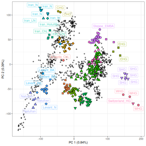

plot of chunk pca_projected_aDNA

Pairwise Fst

Now let’s replicate the pairwise Fst analysis from Lazaridis et al. (2016).

First we need to merge the ancient and modern data:

ancient_modern <- rbind(ho_modern, ancient)
#> harmonising loci between two datasets
#> flip_strand =  FALSE  ; remove_ambiguous =  FALSE 
#> -----------------------------
#> dataset: reference 
#> number of SNPs: 548749 reduced to 548749 
#> ( 0 are ambiguous, of which 0  were removed)
#> -----------------------------
#> dataset: target 
#> number of SNPs: 1233553 reduced to 548749 
#> ( 0 were flipped to match the reference set)
#> ( 36301 are ambiguous, of which 36301 were removed)
#> 
#> gen_tibble saved to /tmp/RtmpptKMxO/gt_merged_42bc4e3e7eb.gt
#> using bigSNP file: /tmp/RtmpptKMxO/gt_merged_42bc4e3e7eb.rds
#> with backing file: /tmp/RtmpptKMxO/gt_merged_42bc4e3e7eb.bk
#> make sure that you do NOT delete those files!
#> to reload the gen_tibble in another session, use:
#> gt_load('/tmp/RtmpptKMxO/gt_merged_42bc4e3e7eb.gt')

Then, we group the ancient and modern data by population:

ancient_modern <- ancient_modern %>% group_by(population)

As we are calculating Fst between populations, we will remove any populations that contain only one individual.

ancient_modern <- ancient_modern %>%
  filter(n() > 1)

And then we can calculate Fst:

pairwise_fst_tidy <- pairwise_pop_fst(ancient_modern,
  method = "Hudson",
  type = "tidy"
)

We can then assign time ranges to the populations based on their names. This will allow us to group populations by time period when creating our plot:

pairwise_fst_tidy <- pairwise_fst_tidy %>%
  mutate(time_range_pop1 = case_when(
    str_detect(population_1, "BA") ~ "Bronze Age",
    str_detect(
      population_1,
      "ChL|_EN|_N|Eneolithic"
    ) ~ "European Neolithic to Chalcolithic",
    str_detect(population_1, "HG|Natufian") ~ "Before European Neolithic",
    TRUE ~ "Present"
  )) %>%
  mutate(time_range_pop2 = case_when(
    str_detect(population_2, "BA") ~ "Bronze Age",
    str_detect(
      population_2,
      "ChL|_EN|_N|Eneolithic"
    ) ~ "European Neolithic to Chalcolithic",
    str_detect(population_2, "HG|Natufian") ~ "Before European Neolithic",
    TRUE ~ "Present"
  ))

After adding the time ranges, we can filter the pairwise Fst data to only include comparisons between populations from the same time range, and set these ranges as factor levels to order the plot:

pairwise_fst_tidy <- pairwise_fst_tidy %>%
  filter(time_range_pop1 == time_range_pop2) %>%
  mutate(time_range_pop1 = factor(time_range_pop1, levels = c(
    "Present",
    "Bronze Age",
    "European Neolithic to Chalcolithic",
    "Before European Neolithic"
  )))

Finally, we will calculate the median, minimum, and maximum values for each time range, so that these can be added to the plot:

medians <- pairwise_fst_tidy %>%
  group_by(time_range_pop1) %>%
  summarise(median_value = median(value, na.rm = TRUE)) %>%
  arrange(factor(time_range_pop1,
    levels = unique(pairwise_fst_tidy$time_range_pop1)
  ))

min <- pairwise_fst_tidy %>%
  group_by(time_range_pop1) %>%
  summarise(min_value = min(value, na.rm = TRUE))

max <- pairwise_fst_tidy %>%
  group_by(time_range_pop1) %>%
  summarise(max_value = max(value, na.rm = TRUE))

We can create our plot using ggplot2, adding the median, minimum, and maximum values as lines and text labels:

ggplot(pairwise_fst_tidy, aes(x = value, y = time_range_pop1)) +
  geom_point() +
  geom_line(
    data = medians, aes(x = median_value, y = time_range_pop1, group = 1),
    color = "red", linewidth = 1.2
  ) +
  geom_text(data = min, aes(
    x = min_value, y = time_range_pop1,
    label = round(min_value, 3), vjust = -0.7
  )) +
  geom_text(data = max, aes(
    x = max_value, y = time_range_pop1,
    label = round(max_value, 3), vjust = -0.7
  )) +
  labs(x = expression("F"[ST]), y = element_blank())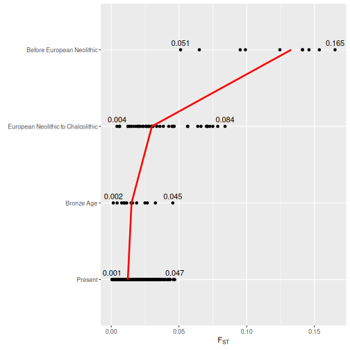

plot of chunk pairwise_fst

F statistics

To calculate F statistics, tidypopgen integrates with the R admixtools package (a.k.a. ADMIXTOOLS 2). The function gt_extract_f2 allows users to calculate blocked f2 statistics from a gen_tibble object, operating in the same way as the extract_f2 function of admixtools.

gt_extract_f2 can be used as follows:

f2s <- gt_extract_f2(ancient_modern,
  outdir = "./data/NearEastPublic/f2"
)

We could now use any of the functions from admixtools giving the outdir with the f2 values.