This vignette is a benchmark of a few key functions in the tidypopgen package. The Human Genome Diversity Project (HGDP) SNP dataset is used for this benchmark. This dataset includes 1043 individuals from 51 populations, typed at ~650k loci.
We will run this benchmark on a machine with a GenuineIntel, 13th Gen
Intel(R) Core(TM) i9-13900, 24 CPU and 126 GiB of RAM. However, we will
limit the number of cores used to 20. Parallelised functions within
tidypopgen use an n_cores argument for the user to set.
However, to prevent a behind-the-scenes inflation of the number of
threads used (for example, in cases where dependency functions may
automatically use all available cores) we need to set up preferences at
the beginning of the session. Specifically, we limit the number of cores
used by the parallelised BLAS library with
bigparallelr::set_blas_ncores(), and by the package
data.table with data.table::setDTthreads().
n_cores <- 20

data.table::setDTthreads(n_cores)
bigparallelr::set_blas_ncores(n_cores)
We can now load the necessary libraries:
And before running the benchmark, we need to download the relevant files. We can use the following to download the HGDP files into a temporary directory:
temp_dir <- tempdir()
download_url <- "https://zenodo.org/records/15582364/files/hgdp650_id_pop.txt"
download_path <- file.path(temp_dir, "hgdp650_id_pop.txt")
download.file(download_url, download_path, mode = "wb")
download_url <- "https://zenodo.org/records/15582364/files/hgdp650.qc.hg19.bed"
download_path <- file.path(temp_dir, "hgdp650.qc.hg19.bed")
download.file(download_url, download_path, method = "wget")
download_url <- "https://zenodo.org/records/15582364/files/hgdp650.qc.hg19.bim"
download_path <- file.path(temp_dir, "hgdp650.qc.hg19.bim")
download.file(download_url, download_path, method = "wget")
download_url <- "https://zenodo.org/records/15582364/files/hgdp650.qc.hg19.fam"
download_path <- file.path(temp_dir, "hgdp650.qc.hg19.fam")
download.file(download_url, download_path, method = "wget")
In the following vignette, we place these files into the subdirectory
data/hgdp/, and we will use the paths to the bed file
hgdp650.qc.hg19.bed and the metadata file
hgdp650_id_pop.txt to read in our data.
bed_path <- "./data/hgdp/hgdp650.qc.hg19.bed"
meta_info <- readr::read_tsv("./data/hgdp/hgdp650_id_pop.txt")
#> Rows: 1064 Columns: 6
#> ── Column specification ──────────────────────────────────────────────────────────────────────────────────────────────────
#> Delimiter: "\t"
#> chr (6): Id, Sex, population, Geographic_origin, Region, Pop7Groups
#>
#> ℹ Use `spec()` to retrieve the full column specification for this data.
#> ℹ Specify the column types or set `show_col_types = FALSE` to quiet this message.
Create gen_tibble object
Our first step is to load the HGDP data into a
gen_tibble object, and add its associated metadata.
hgdp <- gen_tibble(bed_path,
  quiet = TRUE,
  backingfile = tempfile("test_"),
  n_cores = n_cores
)
read_plink: 2.6s
Add metadata
hgdp <- hgdp %>% mutate(
  population = meta_info$population[match(hgdp$id, meta_info$Id)],
  region = meta_info$Region[match(hgdp$id, meta_info$Id)]
)
Let’s confirm that we have read all the expected information:
hgdp
#> # A gen_tibble: 643733 loci
#> # A tibble:     1,043 × 4
#>    id         genotypes population region
#>    <chr>     <vctr_SNP> <chr>      <chr>
#>  1 HGDP00448          1 Biaka_HG   Africa
#>  2 HGDP00479          2 Biaka_HG   Africa
#>  3 HGDP00985          3 Biaka_HG   Africa
#>  4 HGDP01094          4 Biaka_HG   Africa
#>  5 HGDP00982          5 Mbuti_HG   Africa
#>  6 HGDP00911          6 Mandenka   Africa
#>  7 HGDP01202          7 Mandenka   Africa
#>  8 HGDP00927          8 Yoruba     Africa
#>  9 HGDP00461          9 Biaka_HG   Africa
#> 10 HGDP00451         10 Biaka_HG   Africa
#> # ℹ 1,033 more rows
Loci Report
We can then call qc_report_loci. This function supplies
minor allele frequency, rate of missingness, and a Hardy-Weinberg exact
p-value for each SNP.
loci_report <- qc_report_loci(hgdp)
#> This gen_tibble is not grouped. For Hardy-Weinberg equilibrium, `qc_report_loci()` will assume individuals are part of the same population and HWE test p-values will be calculated across all individuals. If you wish to calculate HWE p-values within populations or groups, please use`group_by()` before calling `qc_report_loci()`.
loci_report: 1.8s The resulting report can be observed using
autoplot.
autoplot(loci_report, type = "all")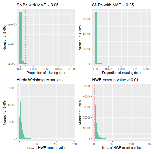
Filter Loci
Following this, we filter the loci to only including those with a minor allele frequency over 0.05, and a missingness rate below 0.05.
to_keep_loci <-
  subset(loci_report, loci_report$maf > 0.05 & loci_report$missingness < 0.05)
hgdp <- hgdp %>% select_loci(to_keep_loci$snp_id)
filter_loci: 1.5s
Individual Report
We can then call qc_report_indiv to supply observed
heterozygosity per individual, and rate of missingness per
individual.
indiv_report <- qc_report_indiv(hgdp)indiv_report: 2.4s
autoplot(indiv_report, type = "scatter")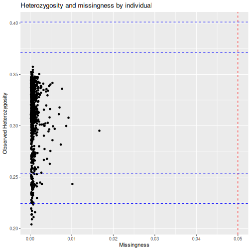
Filter individuals
And we can filter individuals down to only include those with less than 1% of their genotypes missing.
to_keep_indiv <- which(indiv_report$missingness < 0.01)
hgdp <- hgdp[to_keep_indiv, ]
filter_indiv: 4ms
Update backingfile
After removing individuals from the dataset, and before imputing, we
need to update the file backing matrix with
gt_update_backingfile.
hgdp <- gt_update_backingfile(hgdp)
#> Genetic distances are not sorted, setting them to zero
#>
#> gen_backing files updated, now
#> using bigSNP file: /tmp/RtmppmRPhl/test_11da24e07766_v2.rds
#> with backing file: /tmp/RtmppmRPhl/test_11da24e07766_v2.bk
#> make sure that you do NOT delete those files!
Impute data
Some functions, such as loci_ld_clump and the
gt_pca functions, require that there is no missingness in
the dataset, so we use gt_impute_simple to impute any
remaining missing genotypes.
hgdp <- gt_impute_simple(hgdp, method = "mode", n_cores = n_cores)
gt_set_imputed(hgdp, TRUE)
impute: 134ms
LD clumping
LD clumping is then performed to control for linkage disequilibrium.
hgdp <- hgdp %>%
  select_loci_if(loci_ld_clump(genotypes, thr_r2 = 0.2, n_cores = n_cores))
ld_clumping: 3.6s
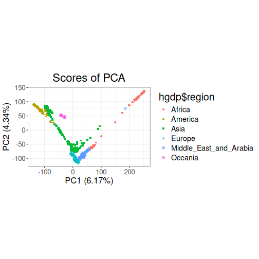
PCA
A principal components analysis can then be computed using the resulting cleaned and LD clumped dataset.
test_pca <- hgdp %>% gt_pca_partialSVD()pca: 1.7s
Plot PCA:
DAPC
We can continue with a discriminant analysis of principal components
using gt_dapc, setting 6 groups corresponding to the main
geographic regions covered by the dataset.
dapc: 35ms
Plot DAPC:
autoplot(test_dapc, type = "scores")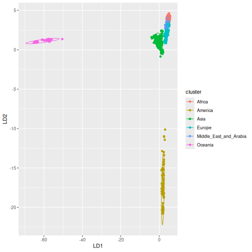
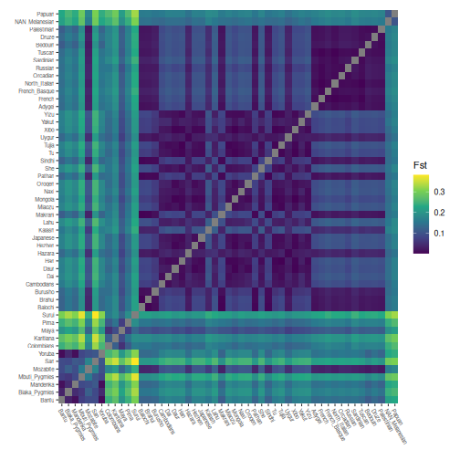
Calculate Fst
To examine the differentiation between populations in the global HGDP set, we calculate pairwise Fst.
grouped_hgdp <- hgdp %>% group_by(population)
pairwise_fsts <- grouped_hgdp %>% pairwise_pop_fst(
  n_cores = n_cores,
  type = "pairwise"
)
pairwise_fst: 3.5s
Plot pairwise Fst:
# Order by continents
grouped_hgdp_order <- grouped_hgdp %>% arrange(region, population)
regional_order <- unique(grouped_hgdp_order$population)
pairwise_fsts <- pairwise_fsts[regional_order, regional_order]

ggheatmap(pairwise_fsts) +
  scale_fill_viridis_c() +
  theme(
    axis.text.x = element_text(angle = -60, hjust = 0, size = 6),
    axis.text.y = element_text(angle = 0, hjust = 1, size = 6)
  ) +
  labs(
    x = element_blank(),
    y = element_blank(),
    fill = "Fst"
  )
Save in plink bed format
Finally, we can save the resulting cleaned dataset to a PLINK .bed file.
gt_as_plink(hgdp,
  file = tempfile(),
  type = "bed",
  overwrite = TRUE
)
#> [1] "/tmp/RtmppmRPhl/file11da6e81448a.bed"
plink_save: 246ms
Summary
Here is a summary of the time taken (in seconds) to perform each step of the analyses:
#>            step  time
#> 1    read_plink  2.61
#> 2   loci_report  1.83
#> 3   filter_loci  1.53
#> 4  indiv_report  2.42
#> 5  filter_indiv     0
#> 6        impute  0.13
#> 7   ld_clumping  3.65
#> 8           pca  1.71
#> 9          dapc  0.03
#> 10 pairwise_fst  3.48
#> 11   plink_save  0.25
#> 12        Total 17.64
Running the benchmark on a laptop
We will now run this benchmark on a laptop with a GenuineIntel, Intel(R) Core(TM) Ultra 7 155H, 22 CPU and 31 GiB of RAM, limiting the number of cores to 4. Here is a summary of the time taken (in seconds) to perform each step of the analyses:
#>            step  time
#> 1    read_plink  4.68
#> 2   loci_report  3.18
#> 3   filter_loci   3.2
#> 4  indiv_report  3.27
#> 5  filter_indiv     0
#> 6        impute  0.88
#> 7   ld_clumping  9.28
#> 8           pca  3.74
#> 9          dapc  0.06
#> 10 pairwise_fst  5.49
#> 11   plink_save  0.34
#> 12        Total 34.12