Find nodes reachable within a cost threshold

The function dijkstraBuffer identifies all nodes reachable from a given origin within a specified maximum cumulative cost, where the distance is defined as the cumulative least-cost path over weighted edges.

Usage

dijkstraBuffer(x, origin, d, res.type = c("nodes", "gGraph"), ...)

Arguments

x

a valid gGraph object with edge costs defined (see setCosts).

origin

either a character string naming a node in x, or a data.frame, list, or numeric vector of length 2 giving longitude and latitude of the origin location.

d

numeric. Maximum cumulative cost defining the reachable area.

res.type

a character string indicating the output format:

• "nodes": a character vector of reachable node names (default).

• "gGraph": the input gGraph with a new logical node attribute reachable indicating which nodes fall within the cost threshold.

...

further arguments passed to other methods (currently unused).

Value

A character vector of reachable node names when res.type = "nodes", or a gGraph object with a new logical node attribute reachable when res.type = "gGraph".

Details

Internally, the function computes single-source shortest paths using Dijkstra's algorithm from the origin node and returns all nodes whose minimum path cost does not exceed the specified threshold.

See also

dijkstraFrom and gPath2dist for the underlying path computations. buffer for geographic distance-based buffers. setCosts to define edge costs before running dijkstraBuffer.

Other dijkstra_methods: dijkstraBetween(), dijkstraFrom(), gPath2dist()

Examples

## Subset gGraph to Europe
x <- rawgraph.10k[isInArea(worldgraph.10k, reg = list(x = c(-10, 50), y = c(35, 70)), quiet = TRUE)]

## Get all nodes reachable within cost 10 from node the origin (here Zurich)
zurich <- data.frame(lon = 8.55, lat = 47.37)

## Set costs for the graph and calculate the buffer
graph <- setCosts(x, attr.name = "habitat", method = "mean")
x2 <- dijkstraBuffer(graph, origin = zurich, d = 10, res.type = "gGraph")

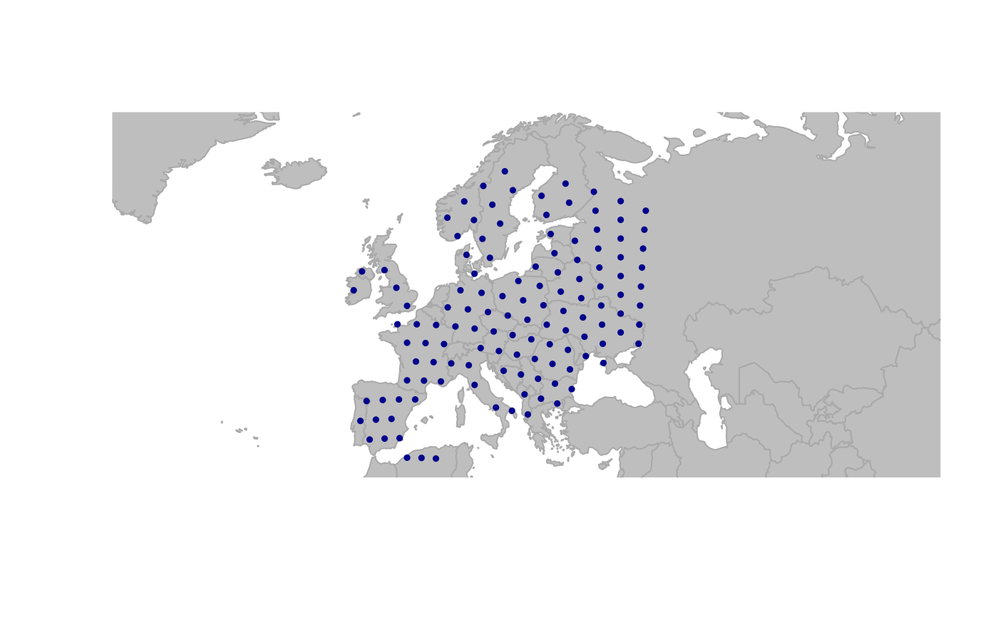
## Plot reachable nodes in dark blue, all others transparent
col.rules <- data.frame(
  reachable = c(TRUE, FALSE),
  color     = c("darkblue", "transparent")
)
plot(x2, col.rules = col.rules, reset = TRUE)
#> Spherical geometry (s2) switched off

#> Spherical geometry (s2) switched on