Manually editing graphs in geoGraph
This vignette will cover the main functions for manually editing
gGraph objects. It also briefly touches on the way
geoGraph keeps track of the plotting area, and how to
navigate within it as some of the interactive functions rely on using
the locator.
Editing gGraphs
Editing graphs is an essential task in geoGraph. While
available gGraph objects provide a basis to work with (see
?worldgraph.10k), one may want to adapt a graph to a
specific case. For instance, connectivity should be defined according to
biological knowledge of the organism under study. gGraph
can be modified in different ways: by changing the connectivity, the
costs of edges, or the attribute values. We already saw in the vignette
‘get started’ how to manually add a connection between two nodes, and we
will see here how to change the global connectivity and edge costs.
Visually inspecting a gGraph object
When customizing a gGraph object, it is often useful to
be able to peer at specific regions, and more generally to navigate
inside the graphical representation of the data. For this, we can use
the interactive functions geo.zoomin,
geo.zoomout, geo.slide, geo.back,
geo.bookmark, and geo.goto. The zoom and slide
functions require to left-click on the graphics to zoom in, zoom out, or
slide to adjacent areas; in all cases, a right click ends the function.
Also note that geo.zoomin can accept an argument specifying
a rectangular region, which will be adapted by the function to fit best
a square area with similar position and center, and zoom to this area
(see ?geo.zoomin). geo.bookmark and
geo.goto respectively set and go to a bookmark,
i.e. a tagged area. This is most useful when one has to switch
between distant areas repeatedly.
Here are some examples based on the plotting of
worldgraph.10k: Zooming in:
plot(worldgraph.10k)
geo.zoomin()
## Spherical geometry (s2) switched off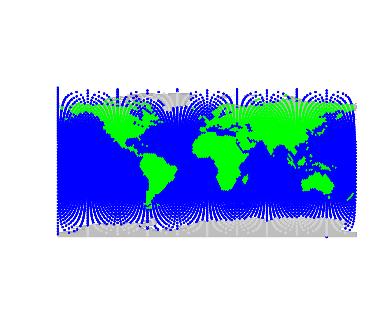
## Spherical geometry (s2) switched on
## Spherical geometry (s2) switched off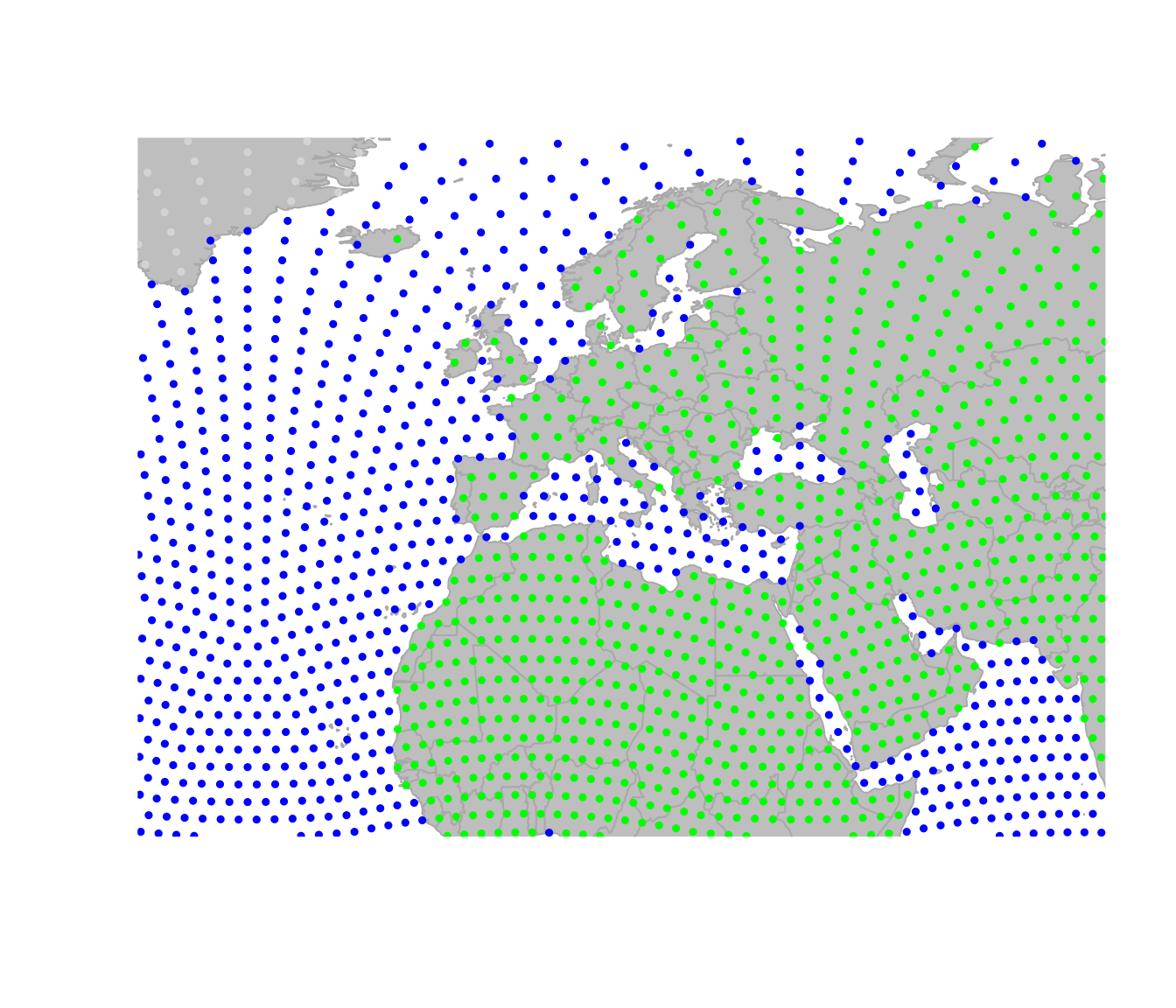
## Spherical geometry (s2) switched onZooming out:
## Spherical geometry (s2) switched off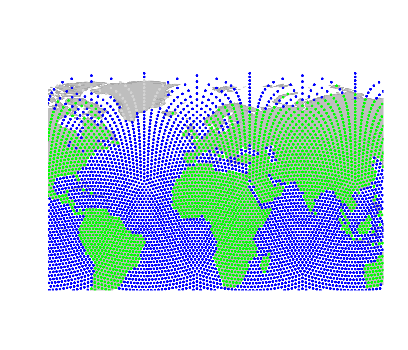
## Spherical geometry (s2) switched onSliding to the east:
## Spherical geometry (s2) switched off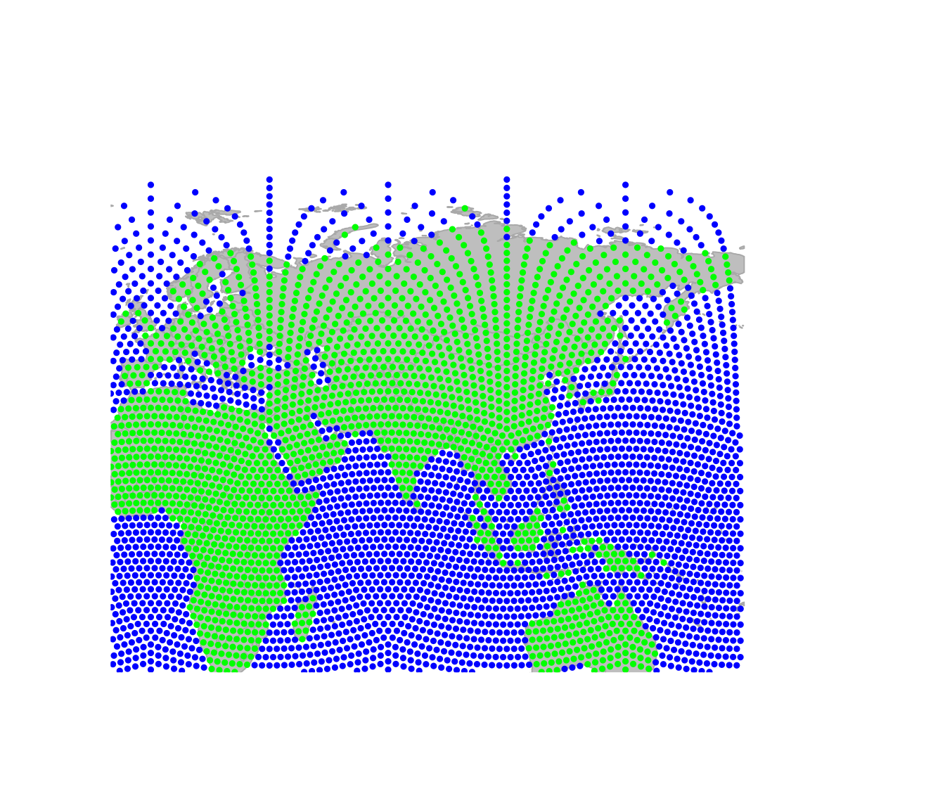
## Spherical geometry (s2) switched onOne important thing which makes plotting gGraph objects
different from most other plotting in R is that geoGraph
keeps the changes made to the plotting area in memory. This allows to
undo one or several moves using geo.back. Moreover, even if
the graphical device is killed, plotting again a gGraph
will use the old parameters by default. To disable this behavior, set
the argument reset=TRUE when calling upon
plot. Technically, this ‘plotting memory’ is implemented by
storing plotting information in an environment defined as the hidden
environment geoGraph:::.geoGraphEnv:
ls(env = geoGraph:::.geoGraphEnv)## [1] "bookmarks" "last.plot" "last.plot.param" "last.points"
## [5] "psize" "sticky.points" "usr" "zoom.log"You can inspect individual variables within this environment:
get("last.plot.param", envir = geoGraph:::.geoGraphEnv)## $psize
## [1] 0.5
##
## $pch
## [1] 19However, it is recommended not to modify these objects directly,
unless you really know what you are doing. In any case, plotting a
gGraph object with argument reset=TRUE will
remove previous plotting history and undo possible wrong
manipulations.
Changing the global connectivity of a gGraph
There are two main ways of changing the connectivity of a
gGraph, which match two different objectives. The first
approach is to perform global and systematic changes of the connectivity
of the graph. Typically, one will want to remove all connections over a
given type of landscape, which is impossible to cross by the organism
under study. Let’s assume we are interested in saltwater fishes. To
model fish dispersal, we have to define a graph which connects only
nodes overlaying the sea. We load the gGraph object
rawgraph.10k, and zoom in to a smaller area (Madagascar) to
illustrate changes in connectivity:
geo.zoomin(c(35, 54, -26, -10))## Spherical geometry (s2) switched off## Spherical geometry (s2) switched on
plotEdges(rawgraph.10k)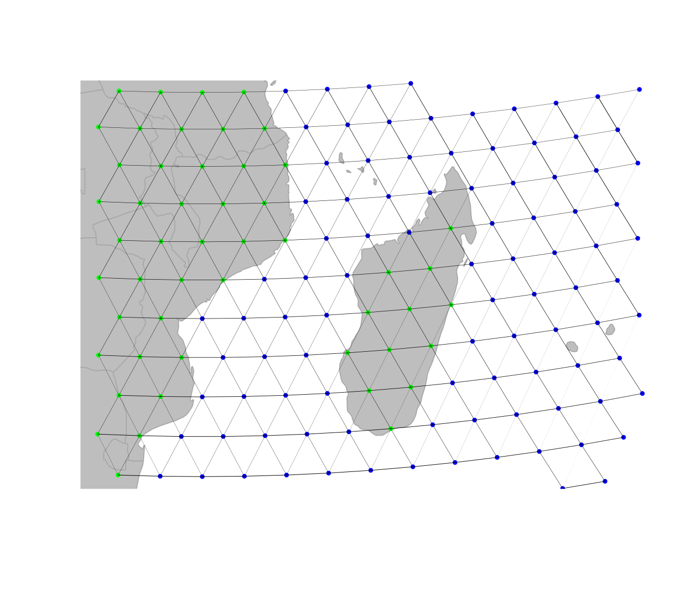
We shall set a bookmark for this area, in case we would want to get back to this place later on:
geo.bookmark("madagascar")##
## Bookmark ' madagascar 'saved.What we now want to do is remove all but sea-sea connections. To do so, the easiest approach is to i) define costs for the edges based on habitat, with land being given large costs and ii) remove all edges with large costs.
Costs of a given node attribute (here, habitat) can be retrieved using getCosts(x, res.type = ‘rules’) and modified using setCosts with the cost.rules argument.
getCosts(rawgraph.10k, res.type = "rules")## habitat cost
## 1 sea 100
## 2 land 1
## 3 mountain 10
## 4 landbridge 5
## 5 oceanic crossing 20
## 6 deselected land 100
cost.rules <- getCosts(rawgraph.10k, res.type = "rules")
cost.rules$cost[cost.rules$habitat == "sea"] <- 1
cost.rules$cost[cost.rules$habitat != "sea"] <- 100
newGraph <- setCosts(rawgraph.10k, attr.name = "habitat", cost.rules = cost.rules)
getCosts(newGraph, res.type = "rules")
## habitat cost
## 1 sea 1
## 2 land 100
## 3 mountain 100
## 4 landbridge 100
## 5 oceanic crossing 100
## 6 deselected land 100We have just changed the costs associated to habitat type, but this
change is not yet effective on edges between nodes. We use
setCosts to set the cost of an edge to the average of the
costs of its nodes:
## Spherical geometry (s2) switched off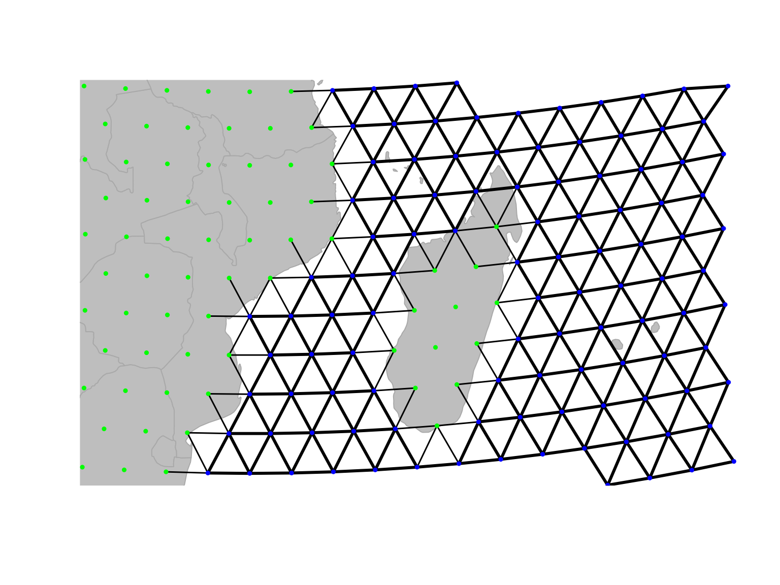
## Spherical geometry (s2) switched onOn this new graph, we represent the edges with a width inversely
proportional to the associated cost; that is, bold lines for easy
traveling and light edges/dotted lines for more costly movement. This is
not enough yet, since traveling on land is still possible. However, we
can tell geoGraph to remove all edges associated to too strong
a cost, as defined by a given threshold (using
dropDeadEdges). Here, only sea-sea connections shall be
retained, that is, edges with cost 1.
newGraph <- dropDeadEdges(newGraph, thres = 1.1)
plot(newGraph, edge = TRUE)
## Spherical geometry (s2) switched off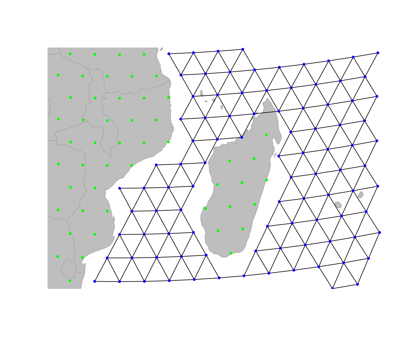
## Spherical geometry (s2) switched onHere we are: newGraph only contains connections in the
sea. Note that, although we restrained the plotting area to Madagascar,
this change is effective everywhere. For instance, traveling to the
north-west Australian coasts:
geo.zoomin(c(110, 130, -27, -12))## Spherical geometry (s2) switched off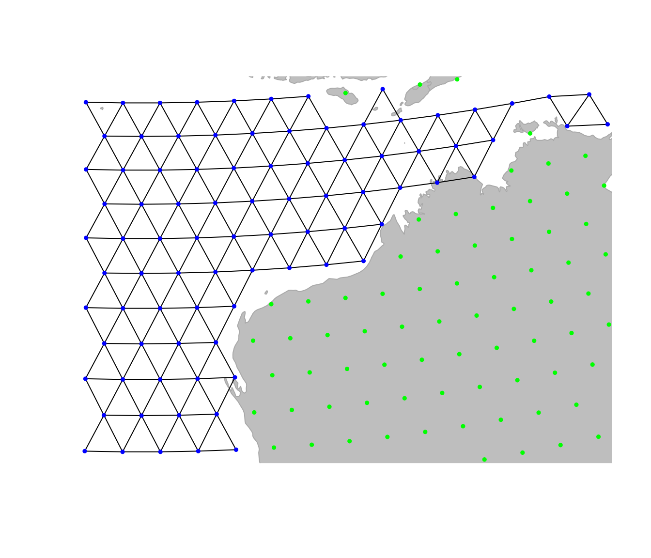
## Spherical geometry (s2) switched on
geo.bookmark("australia")##
## Bookmark ' australia 'saved.Changing local properties of a gGraph
A second approach to changing a gGraph is to refine the
graph by hand, adding or removing locally some connections, or altering
the attributes of some nodes. This can be necessary to connect
components such as islands to the main landmasses, or to correct
erroneous data. As seen in the vignette ‘get started’, adding and
removing edges from the grid of a gGraph can be achieved by
geo.add.edges and geo.remove.edges,
respectively. These functions are interactive, and require the user to
select individual nodes or a rectangular area in which edges are added
or removed. See ?geo.add.edges for more information on
these functions. For instance, we can remove a few odd connections in
the previous graph, near the Australian coasts (note that we have to
save the changes using <-):
geo.goto("australia")
newGraph <- geo.remove.edges(newGraph)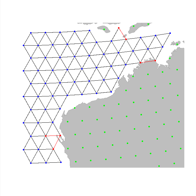
When adding connections within an area or in an entire graph, node
addition is based on another gGraph, i.e. only
connections existing in another gGraph serving as reference
can be added to the current gGraph. For graphs based on 10k
or 40k grids, the raw graphs provided in geoGraph should be
used, (rawgraph.10k, rawgraph.40k), since they
are fully connected.
In addition to changing grid connectivity, we may also want to modify
the attributes of specific nodes. This is again done interactively,
using the function geo.change.attr. For instance, here, we
define a new value shallowwater (plotted in light blue) for
the attribute habitat, selecting affected nodes using the
‘area’ mode first, and refining the changes using the ‘point’ mode:
plot(newGraph, edge = TRUE)
newGraph <- geo.change.attr(newGraph,
  mode = "area", attr.name = "habitat",
  attr.value = "shallowwater", newCol = "deepskyblue"
)
newGraph <- geo.change.attr(newGraph,
  attr.name = "habitat",
  attr.value = "shallowwater", newCol = "deepskyblue"
)
getColors(newGraph, res.type = "rules")## habitat color
## 1 sea blue
## 2 land green
## 3 mountain brown
## 4 landbridge light green
## 5 oceanic crossing light blue
## 6 deselected land lightgray
## 7 shallowwater deepskyblue
plot(newGraph, edge = TRUE)## Spherical geometry (s2) switched off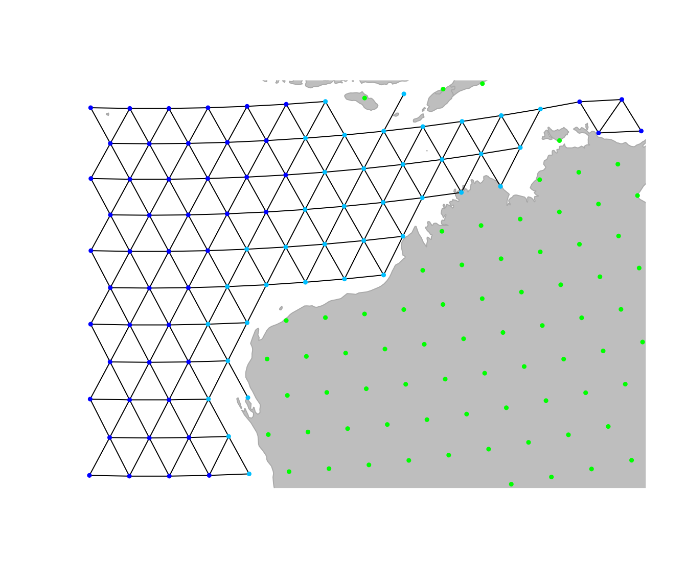
## Spherical geometry (s2) switched onAgain, note that the changes made to the graph have to be saved in an
object (using <-) to be effective.