geoGraph

2026-09-07

geoGraph: using spherical grids to walk through the geographic space

In this vignette, we go through the basic tasks that can be achieved using geoGraph. A short overview of the functionality of the package is summarized the package’s manpage, accessible via:

?geoGraph

geoGraph aims at implementing graph approaches for geographic data. In geoGraph, a given geographic area is modeled by a fine regular grid, where each vertex has a set of spatial coordinates and a set of attributes, which can be for instance habitat descriptors, or the presence/abundance of a given species. ‘traveling’ within the geographic area can then be easily modeled as moving between connected vertices. The cost of moving from one vertex to another can be defined according to attribute values, which allows for instance to define friction routes based on habitat.

geoGraph harnesses the full power of graph algorithms implemented in R by the graph and RBGL (R Boost Graph Library) packages. In particular, RBGL is an interface between R and the comprehensive Boost Graph Library in C++, which provides fast and efficient implementations of a wide range of graph algorithms. Once we have defined frictions for an entire geographic area, we can easily, for instance, find the least costs path from one location to another, or find the most parsimonious way of connecting a set of locations.

Interfacing spatial data and graphs can be a complicated task. The purpose of geoGraph is to provide tools to achieve and simplify this ‘preliminary’ step. This is achieved by defining new classes of objects which are essentially geo-referenced graphs with node attributes (gGraph objects), and interfaced spatial data (gData objects). In this vignette, we show how to install geoGraph, construct and handle gGraph/gData objects, and illustrate some basic features of graph algorithms.

First steps

Installing the package

All the following instructions should be entered from a new R session to avoid errors due to installing attached packages.

You can install geoGraph from GitHub with:

install.packages("pak")
pak::pak("EvolEcolGroup/geograph")

Once installed, the package can be loaded using:

library("geoGraph")

If you have an error regarding missing packages, you may need to install manually the packages graph and RBGL from Bioconductor:

install.packages("BiocManager")
BiocManager::install(c("graph", "RBGL"))

And then attempt to reinstall geoGraph from GitHub.

Data representation

Data representation refers to the way a given type of data is handled by a computer program. Two types of objects are used in geoGraph: gGraph, and gData objects. Both objects are defined as formal (S4) classes and often have methods for similar generic function (e.g. getNodes is defined for both objects). Essentially, gGraph objects contain underlying layers of information, including a spatial grid and possibly node attributes. gData are sets of locations (like sampled sites, for instance) which have been interfaced to a gGraph object, to allow further manipulations such as finding paths on the grid between pairs of locations.

gGraph objects

The definition of the formal class gGraph can be obtained using:

getClass("gGraph")

## Class "gGraph" [package "geoGraph"]
## 
## Slots:
##                                                   
## Name:      coords nodes.attr       meta      graph
## Class:     matrix data.frame       list   graphNEL

and a new empty object can be obtained using the constructor:

new("gGraph")

## 
## === gGraph object ===
## 
## @coords: spatial coordinates of 0 nodes
##      lon lat
## 
## @nodes.attr: 0 nodes attributes
## data frame with 0 columns and 0 rows
## 
## @meta: list of meta information with 0 items
## 
## @graph:
## A graphNEL graph with undirected edges
## Number of Nodes = 0 
## Number of Edges = 0

The documentation ?gGraph explains the basics about the object’s content. In a nutshell, these objects are spatial grids with nodes and segments connecting neighboring nodes, and additional information on the nodes or on the graph itself. coords is a matrix of longitudes and latitudes of the nodes. nodes.attr is a data.frame storing attributes of the nodes, such as habitat descriptors; each row corresponds to a node of the grid, while each column corresponds to a variable. meta is a list containing miscellaneous information about the graph itself. There is no constraint applying to the components of the list, but some typical components such as $costs or $colors will be recognized by certain functions. For instance, you can specify plotting rules for representing a given node attribute by a given color by defining a component $colors. Similarly, you can associate costs to a given node attribute by defining a component $costs. An example of this can be found in already existing gGraph objects. For instance, worldgraph.10k is a graph of the world with approximately 10,000 nodes, and only on-land connectivity i.e. no traveling on the seas.

worldgraph.10k@meta

## $colors
##            habitat       color
## 1              sea        blue
## 2             land       green
## 3         mountain       brown
## 4       landbridge light green
## 5 oceanic crossing  light blue
## 6  deselected land   lightgray
## 
## $costs
##            habitat cost
## 1              sea  100
## 2             land    1
## 3         mountain   10
## 4       landbridge    5
## 5 oceanic crossing   20
## 6  deselected land  100

Lastly, the graph component is a graphNEL object, which is the standard class for graphs in the graph and RBGL packages. This object contains all information on the connections between nodes, and the weights (costs) of these connections.

Four main gGraph are provided with geoGraph: rawgraph.10k, rawgraph.40k, worldgraph.10k, and worldgraph.40k. These datasets are available using the command data. The grid used in these datasets are the best geometric approximation of a regular grid for the surface of a sphere. One advantage of working with these grids is that we do not have to use a projection for geographic coordinates, which is a usual issue in regular GIS.

The difference between rawgraphs and worldgraphs is that the first are entirely connected, while in the second connections occur only on land. Numbers 10k' and40k’ indicate that the grids consist of roughly 10,000 and 40,000 nodes. For illustrative purposes, we will often use the 10k grids, since they are less heavy to handle. For most large-scale applications, the 40k versions should provide sufficient resolution. New gGraph can be constructed using the constructor (new(...)). A more detailed description of how to construct custom gGraph is provided in the vignette ‘Making custom grids in geoGraph’ (see vignette() for more information on available vignettes).

gData objects

gData objects store sets of locations interfaced with a gGraph object. When creating a gData, each location is matched to its closest node on the gGraph grid, which makes it possible to model travel between locations along the grid — for instance, to find the shortest path between two sites through different habitat types.

Like for gGraph, the content of the formal class gData can be obtained using:

getClass("gData")

## Class "gData" [package "geoGraph"]
## 
## Slots:
##                                                       
## Name:       coords    nodes.id        data gGraph.name
## Class:      matrix   character         ANY   character

and a new empty object can be obtained using the constructor:

new("gData")

## 
## === gData object ===
## 
## @coords: spatial coordinates of 0 nodes
##      lon lat
## 
## @nodes.id: 0 nodes identifiers
## character(0)
## 
## @data: data
## NULL
## 
## Associated gGraph:

As before, the description of the content of these objects can be found in the documentation (?gData). coords is a matrix of xy (longitude/latitude) coordinates in which each row is a location. nodes.id is a vector of characters giving the name of the vertices matching the locations; this is defined automatically when creating a new gData, or using the function closestNode. data is a slot storing data associated to the locations; it can be any type of object, but a data.frame should cover most requirements for storing data. Note that this object should be subsettable (i.e. the [ operator should be defined), so that data can be subsetted when subsetting the gData object. Lastly, the slot gGraph.name contains the name of the gGraph object to which the gData has been interfaced.

In the next sections, we illustrate how we can build and use gData objects from a set of locations.

Getting started with geoGraph

Importing geographic data

GeoGraphic data consist of a set of locations, possibly accompanied by additional information. For instance, one may want to study the migrations among a set of biological populations with known geographic coordinates. In geoGraph, geographic data are stored in gData objects. These objects match locations to the closest nodes on a grid (a gGraph object), and store additional data if needed.

As a toy example, let us consider four locations: Bordeaux in France, Berlin in Germany, Baku in Azerbaijan, and Timbuktu in Mali. Since we will be working with a crude grid (10,000 nodes), locations need not be exact.
We enter the longitudes and latitudes (in this order, that is, xy coordinates) of these cities in decimal degrees, as well as approximate population sizes:

bordeaux <- c(-1, 45)
berlin <- c(13, 52)
baku <- c(44, 40)
timbuktu <- c(-3, 16)

cities.dat <- rbind.data.frame(bordeaux, berlin, baku, timbuktu)
colnames(cities.dat) <- c("lon", "lat")
row.names(cities.dat) <- c("Bordeaux", "Berlin", "Baku", "Timbuktu")
cities.dat$pop <- c(250000, 3500000, 2000000, 50000)
cities.dat

##          lon lat     pop
## Bordeaux  -1  45  250000
## Berlin    13  52 3500000
## Baku      44  40 2000000
## Timbuktu  -3  16   50000

We load a gGraph object which contains the grid that will support the data:

plot(worldgraph.10k)

## Spherical geometry (s2) switched off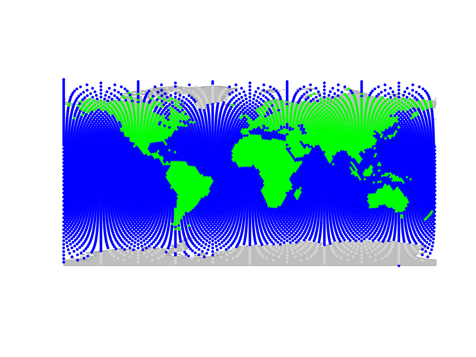

## Spherical geometry (s2) switched on

In this figure, each node is represented with a color depending on the habitat type, either ‘sea’ (blue) or ‘land’ (green). We are going to interface the cities data with this grid; to do so, we create a gData object using new (see ?gData object):

cities <- new("gData", coords = cities.dat[, 1:2], data = cities.dat[, 3, drop = FALSE], gGraph.name = "worldgraph.10k")
cities

## 
## === gData object ===
## 
## @coords: spatial coordinates of 4 nodes
##   lon lat
## 1  -1  45
## 2  13  52
## 3  44  40
## ...
## 
## @nodes.id: 4 nodes identifiers
##      1      2      3 
## "5774" "7696" "2629" 
## ...
## 
## @data: 4 data
##              pop
## Bordeaux  250000
## Berlin   3500000
## Baku     2000000
## ...
## 
## Associated gGraph: worldgraph.10k

plot(cities, type = "both", reset = TRUE)

## Spherical geometry (s2) switched off

## Spherical geometry (s2) switched on

plotEdges(worldgraph.10k)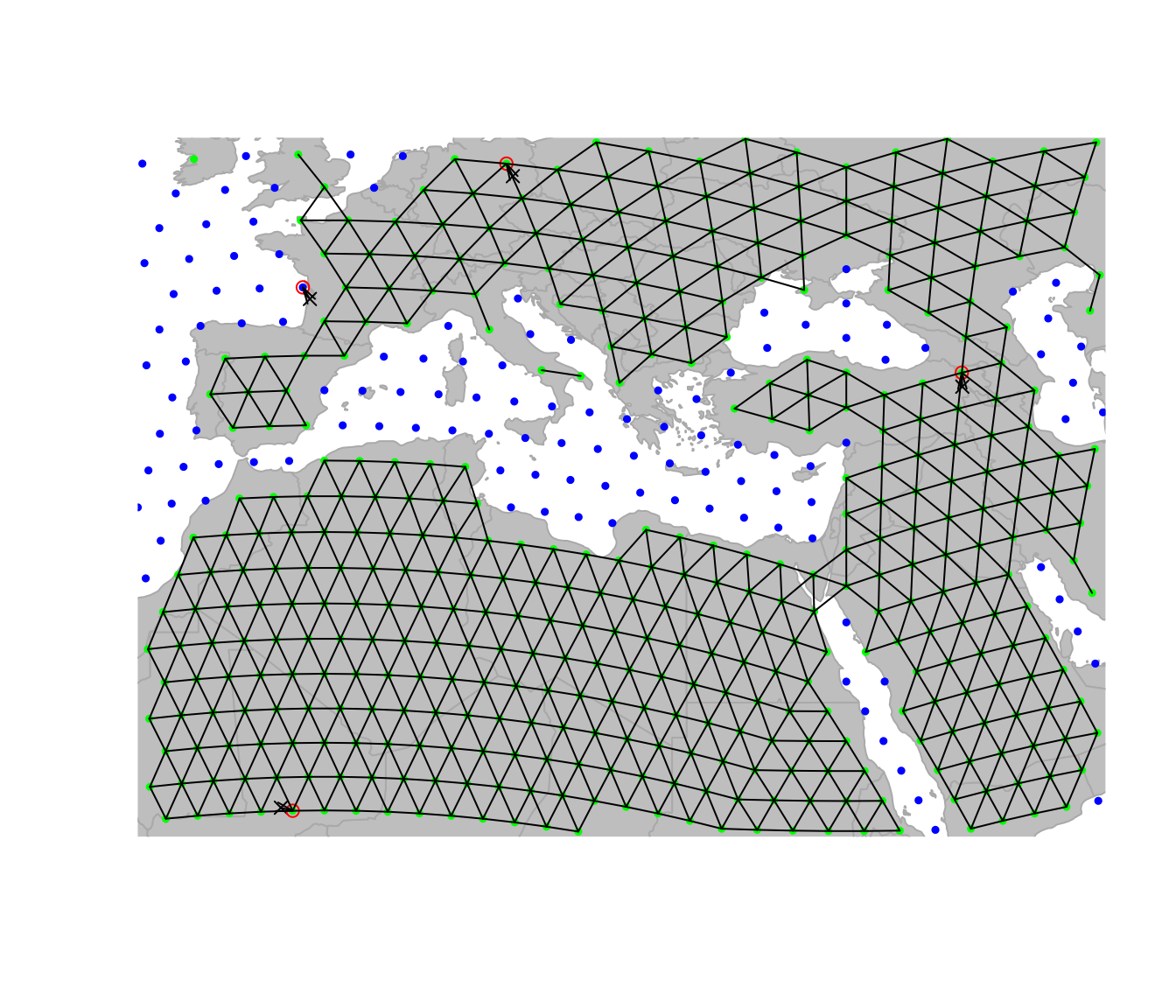

This figure illustrates the matching of original locations (black crosses) to nodes of the grid (red circles). As we can see, an issue occurred for Bordeaux, which has been assigned to a node in the sea (in blue). Locations can be re-assigned to nodes with restrictions for some node attribute values using closestNode; for instance, here we constrain matching nodes to have an habitat value (defined as node attribute in worldgraph.10k) equaling land (green points):

cities <- closestNode(cities, attr.name = "habitat", attr.value = "land")
plot(cities, type = "both", reset = TRUE)

## Spherical geometry (s2) switched off

## Spherical geometry (s2) switched on

plotEdges(worldgraph.10k)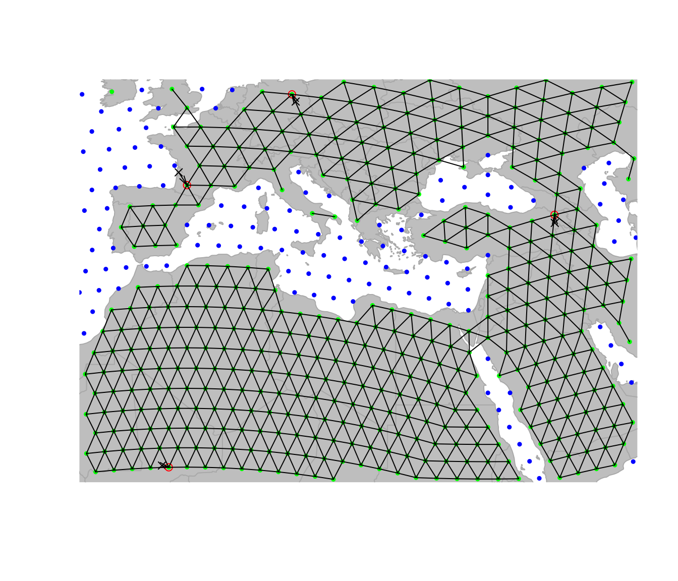

Now, all cities have been assigned to a land node of the grid. Content of cities can be accessed via various accessors (see ?gData). For instance, we can retrieve original locations, assigned nodes, and stored data using:

getCoords(cities)

##      lon lat
## 5775  -1  45
## 7696  13  52
## 2629  44  40
## 3221  -3  16

getNodes(cities)

##   5774   7696   2629   3221 
## "5775" "7696" "2629" "3221"

getData(cities)

##              pop
## Bordeaux  250000
## Berlin   3500000
## Baku     2000000
## Timbuktu   50000

More interestingly, we can now retrieve all the geographic information contained in the underlying grid (i.e. gGraph object) as node attributes:

getNodesAttr(cities)

##      habitat
## 5775    land
## 7696    land
## 2629    land
## 3221    land

In this example, the information stored in worldgraph.10k is rather crude: habitat only distinguishes the land from the sea.

Finding least-cost paths

One of the most useful applications of geoGraph is the research of least-cost paths between couples of locations. This can be achieved using the functions dijkstraFrom and dijkstraBetween on a gData object which contains all the locations of interest. These functions return least-cost paths with the format gPath. dijkstraFrom compute the paths from a given node of the grid to all locations of the gData, while dijkstraBetween computes the paths between pairs of locations of the gData. Below, we illustrate the use of dijkstraBetween to find the least-cost paths between all pairs of cities in our example.

First, we check that all populations are connected on the grid using isConnected:

isConnected(cities)

## [1] TRUE

If not all locations are connected, connectivityPlot can help diagnose the problem by displaying connected components in different colors, and is available for both gGraph and gData objects. For instance:

connectivityPlot(worldgraph.10k, edges = TRUE, seed = 1, reset = TRUE)

## Spherical geometry (s2) switched off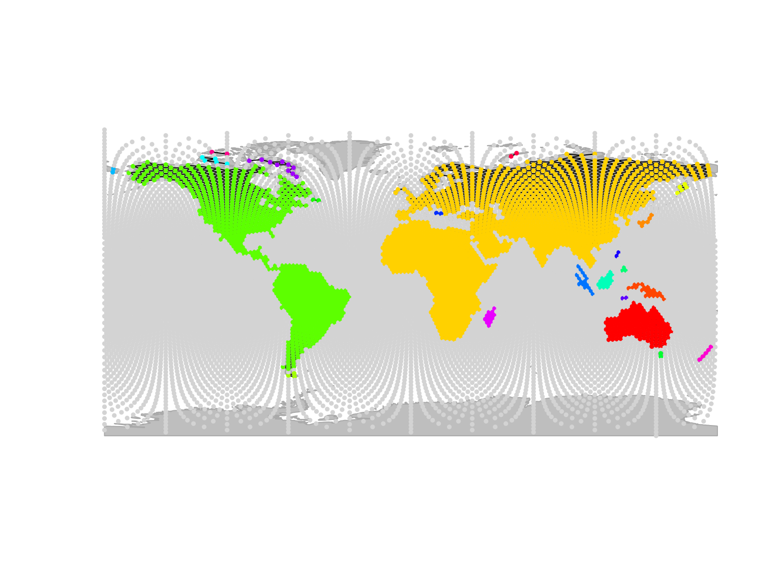

## Spherical geometry (s2) switched on

Since all locations in cities are connected, we can proceed further.

We can now compute least-cost paths between all pairs of cities using dijkstraBetween:

cities.paths <- dijkstraBetween(cities)
cities.paths

## 
## === gPath object ===
## 
##  number of paths: 6 
## 
##  available paths (id_origin:id_destination): 5775:7696 5775:2629 5775:3221 ...
## 
## each path, accessible with [[]] has elements 'length', 'path_detail' and 'length_detail'
## x and y coordinates of all nodes are stored as an attribute 'xy'; see ?gPath for details

plot(cities, reset = TRUE)

## Spherical geometry (s2) switched off

## Spherical geometry (s2) switched on

plot(cities.paths)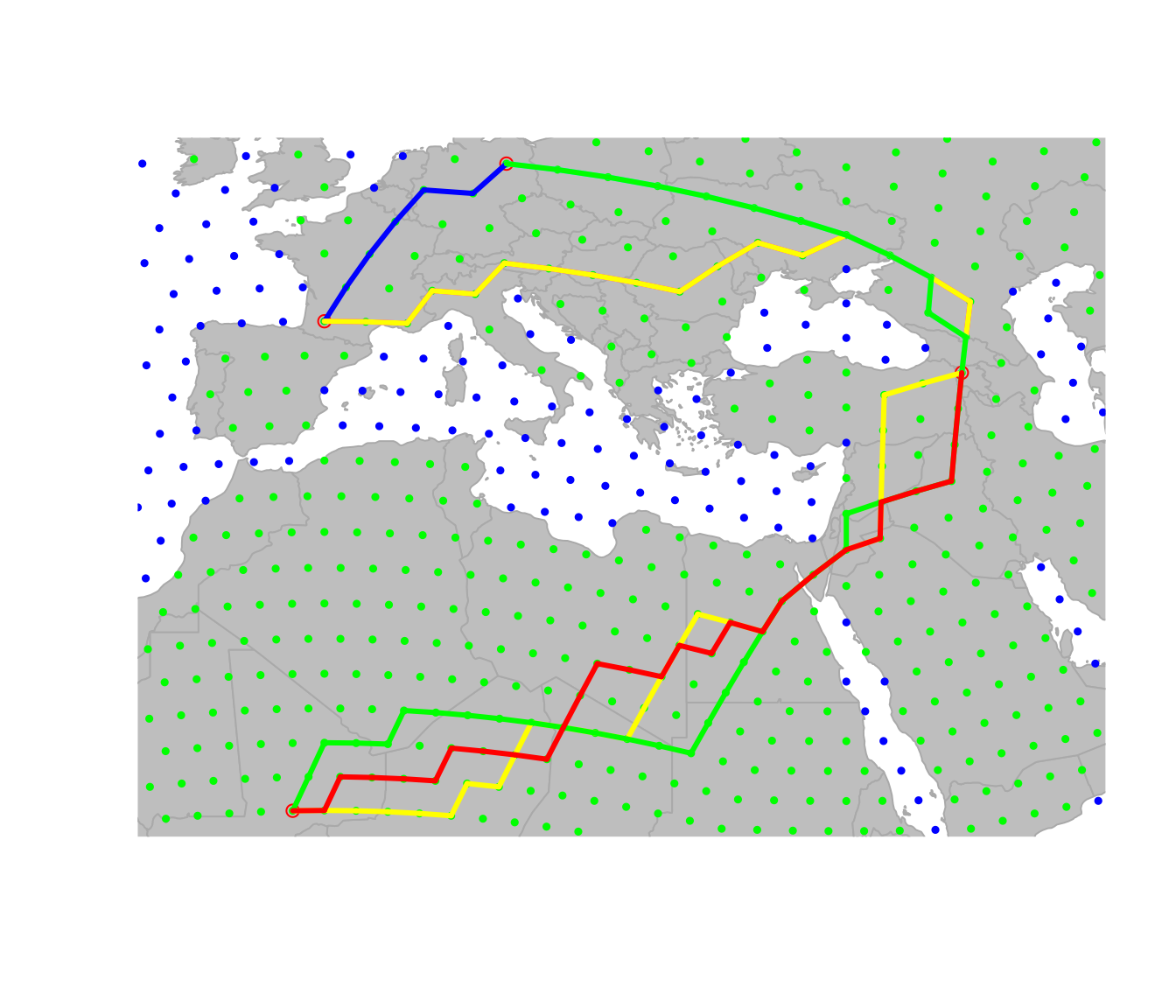

In this graph, each path is plotted with a different color, but several paths overlap in several places. We can clearly see that all paths go through the Caucasus mountains, which is the only land connection between Europe and Africa in this grid. Depending on the application, this may be a problem, since the Strait of Gibraltar is a more likely route for traveling between these two continents. In the next section, we show how to change local properties of a gGraph to allow for a connection at the Strait of Gibraltar.

Changing local properties of a gGraph

In the current version of worldgraph.10k, there is no connection at the Strait of Gibraltar as the grid is designed to only allow for land to land connectivity. We can visually check this by zooming in on the area of interest and plotting the edges of the grid:

geo.zoomin(c(-10, 2, 32, 40))

## Spherical geometry (s2) switched off

## Spherical geometry (s2) switched on

plotEdges(worldgraph.10k)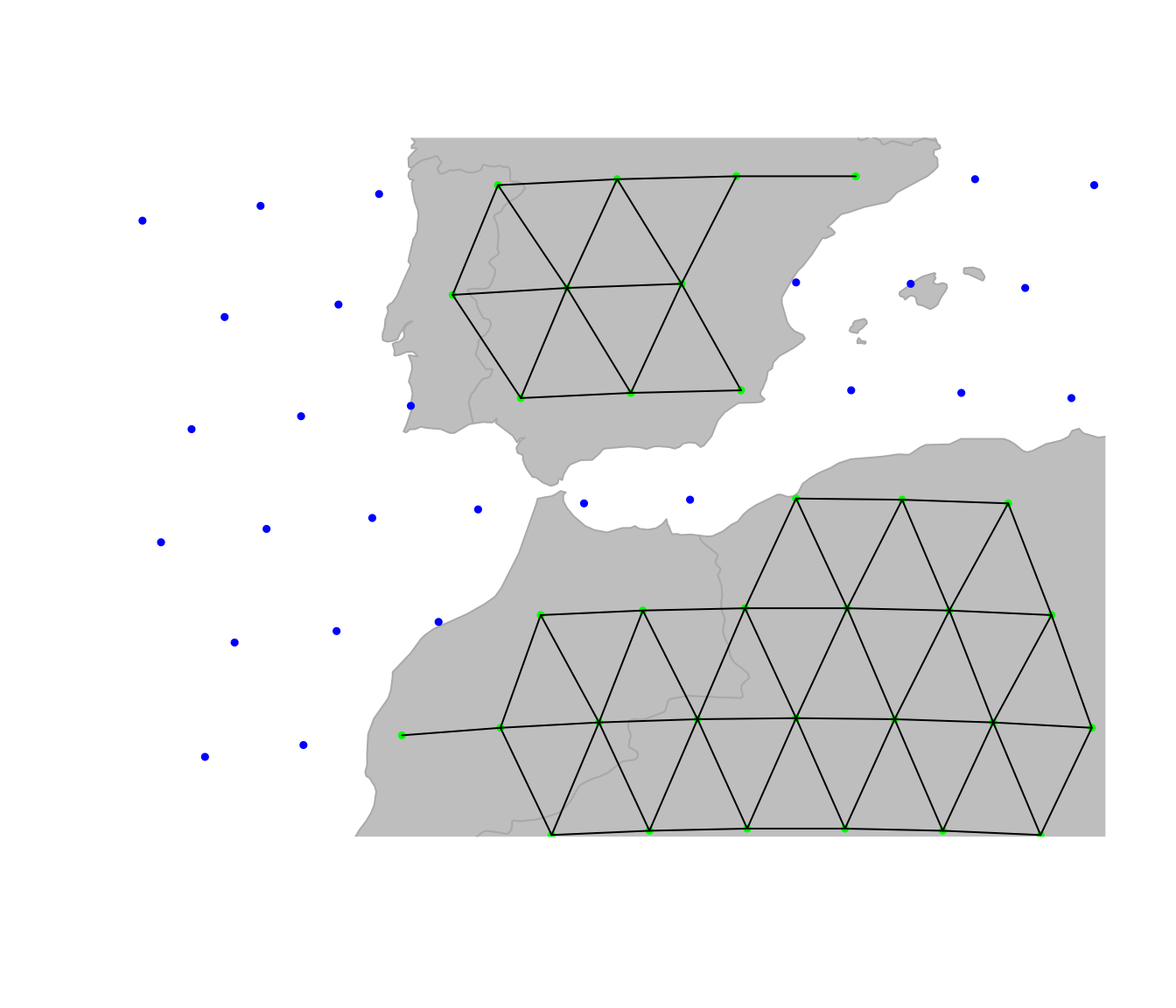

We can change this by adding a connection between the two continents, for instance by adding a connection between the two nodes of the grid which are closest to the Strait of Gibraltar. Adding and removing edges from the grid of a gGraph can be achieved by geo.add.edges and geo.remove.edges, respectively. These functions are interactive, and require the user to select individual nodes or a rectangular area in which edges are added or removed. See ?geo.add.edges for more information on these functions. For instance, we can add the above-mentioned connection between Europe and Africa by selecting the two nodes of the grid closest to the Strait of Gibraltar, and adding a connection between them. For this we just run the ‘geo.add.edges’ function, and then click on the two nodes of the grid that we want to connect (in this case, one node in Europe and one node in Africa). After adding the edge, we can save the new graph as a new object (note that we have to save the changes using <-):

newGraph <- worldgraph.10k
plot(newGraph)
newGraph <- geo.add.edges(newGraph)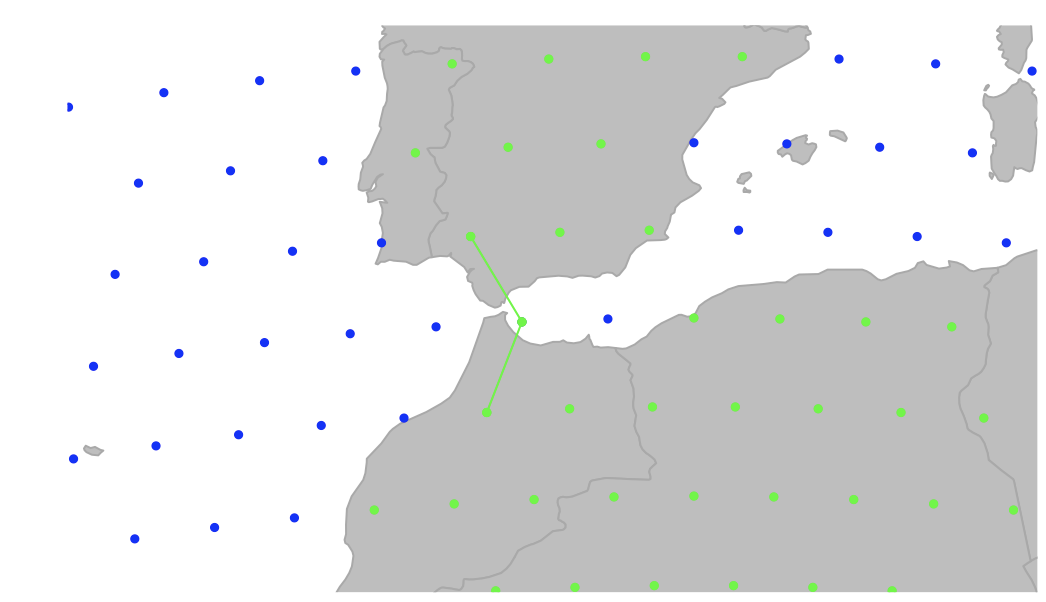

img

We can then assign the new graph using the setGraph function, so that the new graph will be used for path computations. Now when we compute least-cost paths between cities, we can see that the path between Bordeaux and Timbuktu goes through the Strait of Gibraltar instead of the Caucasus mountains:

cities <- setGraph(cities, "newGraph")
cities.paths <- dijkstraBetween(cities)
plot(cities, reset = TRUE)

## Spherical geometry (s2) switched off

## Spherical geometry (s2) switched on

plot(cities.paths)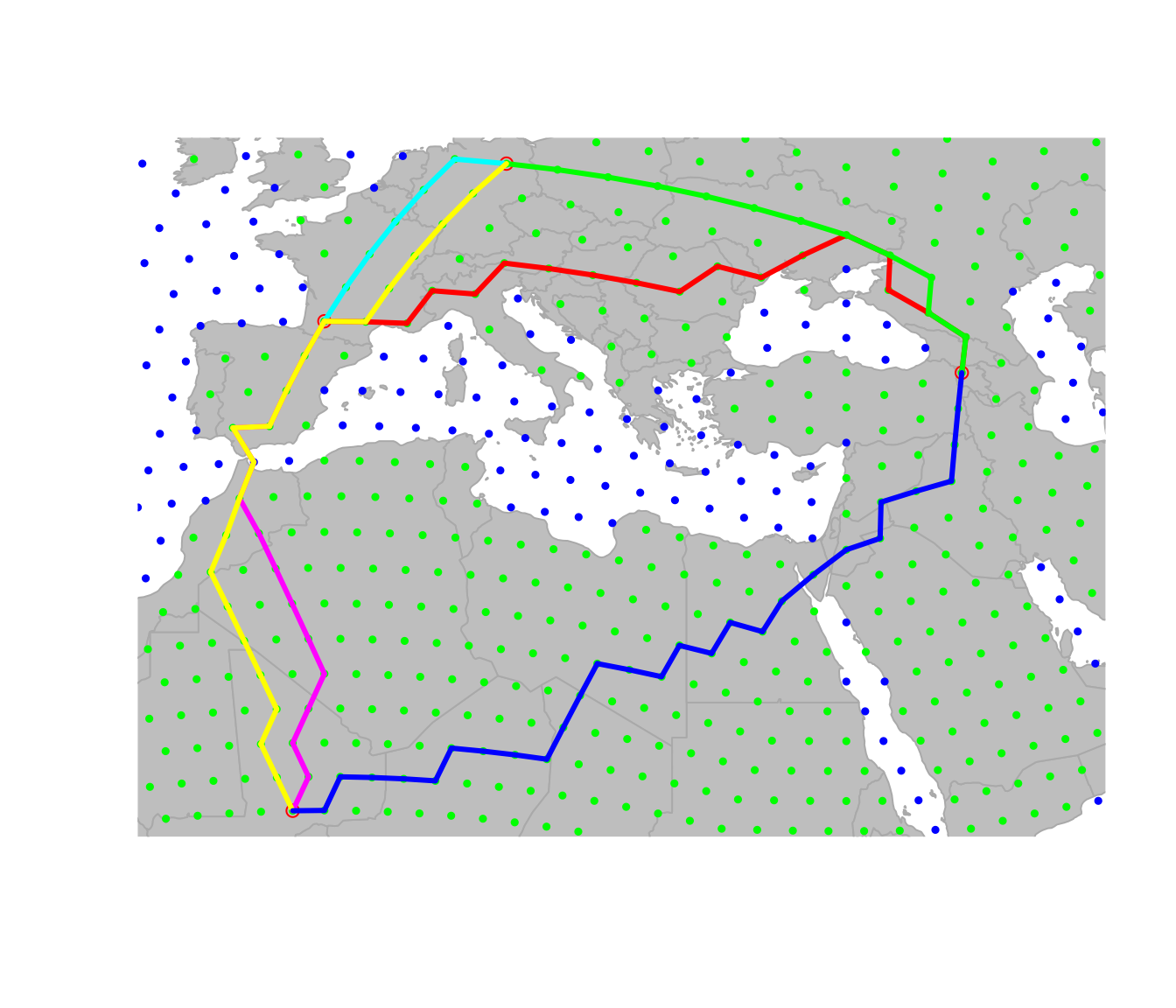

Example application using the Human Genome Diversity Panel

Here we show an application of the above-described methods to a real dataset, the Human Genome Diversity Panel (HGDP) dataset, which contains genetic diversity information for 51 human populations worldwide (see ?hgdp for more information on this dataset).

hgdp

## 
## === gData object ===
## 
## @coords: spatial coordinates of 51 nodes
##   lon lat
## 1  -3  59
## 2  39  44
## 3  40  61
## ...
## 
## @nodes.id: 51 nodes identifiers
##   28179   11012   22532 
## "26898" "11652" "22532" 
## ...
## 
## @data: 51 data
##   Population Region Label  n Latitude Longitude Genetic.Div
## 1   Orcadian EUROPE     1 15       59        -3      0.7259
## 2     Adygei EUROPE     2 17       44        39      0.7298
## 3    Russian EUROPE     3 25       61        40      0.7320
## ...
## 
## Associated gGraph: worldgraph.40k

plot(hgdp, reset = TRUE)

## Spherical geometry (s2) switched off

## Spherical geometry (s2) switched on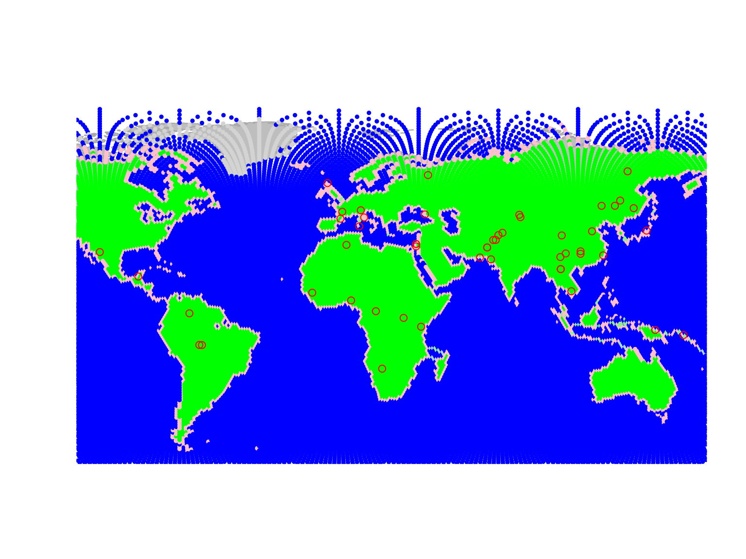

Populations of the dataset are shown by red circles, while the underlying grid (worldgraph.40k) is represented with colors depending on habitat (blue: sea; green: land; pink: coasts). Population genetics predicts that genetic diversity within populations should decay as populations are located further away from the geographic origin of the species. Here, we verify this relationship for a theoretical origin in Addis Ababa, Ethiopia. We shall seek all paths through landmasses to the HGDP populations.

First, we check again that all populations are connected on the grid using isConnected:

isConnected(hgdp)

## [1] TRUE

Since all locations in hgdp are connected, we can proceed further. We have to set the costs of edges in the gGraph grid. To do so, we can choose between i) strictly uniform costs (using dropCosts) ii) distance-based costs – roughly uniform – (using setDistCosts) or iii) attribute-driven costs (using setCosts).

We shall first illustrate the strictly uniform costs. After setting a gGraph with uniform costs, we use dijkstraFrom to find the shortest paths between Addis Ababa and the populations of hgdp:

myGraph <- dropCosts(worldgraph.40k)
hgdp <- setGraph(hgdp, "myGraph")
addis <- cbind(38, 9)
ori <- closestNode(myGraph, addis)
paths <- dijkstraFrom(hgdp, ori)

The object paths contains the identified paths, which are stored as a list with class gPath (see ?gPath). Paths can be plotted easily:

addis <- as.vector(addis)
plot(myGraph, col = NA, reset = TRUE)

## Spherical geometry (s2) switched off

## Spherical geometry (s2) switched on

plot(paths)
points(addis[1], addis[2], pch = "x", cex = 2)
text(addis[1] + 35, addis[2], "Addis Ababa", cex = .8, font = 2)
points(hgdp, col.nodes = "black")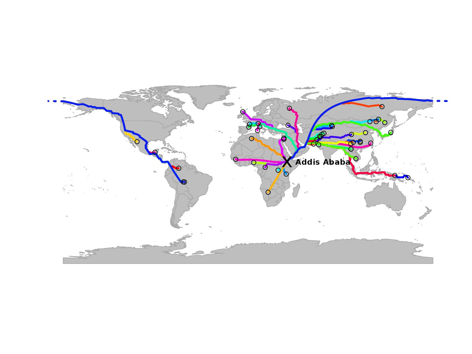

In this graph, each path is plotted with a different color, but several paths overlap in several places. We can extract the distances from the origin using gPath2dist, and then examine the relationship between genetic diversity within populations (stored in hgdp) and the distance from the origin:

div <- getData(hgdp)$"Genetic.Div"
dgeo.unif <- gPath2dist(paths)
plot(div ~ dgeo.unif, xlab = "GeoGraphic distance (arbitrary units)", ylab = "Genetic diversity")
lm.unif <- lm(div ~ dgeo.unif)
abline(lm.unif, col = "red")
summary(lm.unif)

## 
## Call:
## lm(formula = div ~ dgeo.unif)
## 
## Residuals:
##      Min       1Q   Median       3Q      Max 
## -0.07323 -0.00659  0.00075  0.01027  0.05454 
## 
## Coefficients:
##              Estimate Std. Error t value Pr(>|t|)    
## (Intercept)  7.70e-01   4.64e-03   165.8   <2e-16 ***
## dgeo.unif   -8.39e-04   5.36e-05   -15.7   <2e-16 ***
## ---
## Signif. codes:  0 '***' 0.001 '**' 0.01 '*' 0.05 '.' 0.1 ' ' 1
## 
## Residual standard error: 0.0187 on 49 degrees of freedom
## Multiple R-squared:  0.833,  Adjusted R-squared:  0.83 
## F-statistic:  245 on 1 and 49 DF,  p-value: <2e-16

title("Genetic diversity vs geographic distance \n uniform costs ")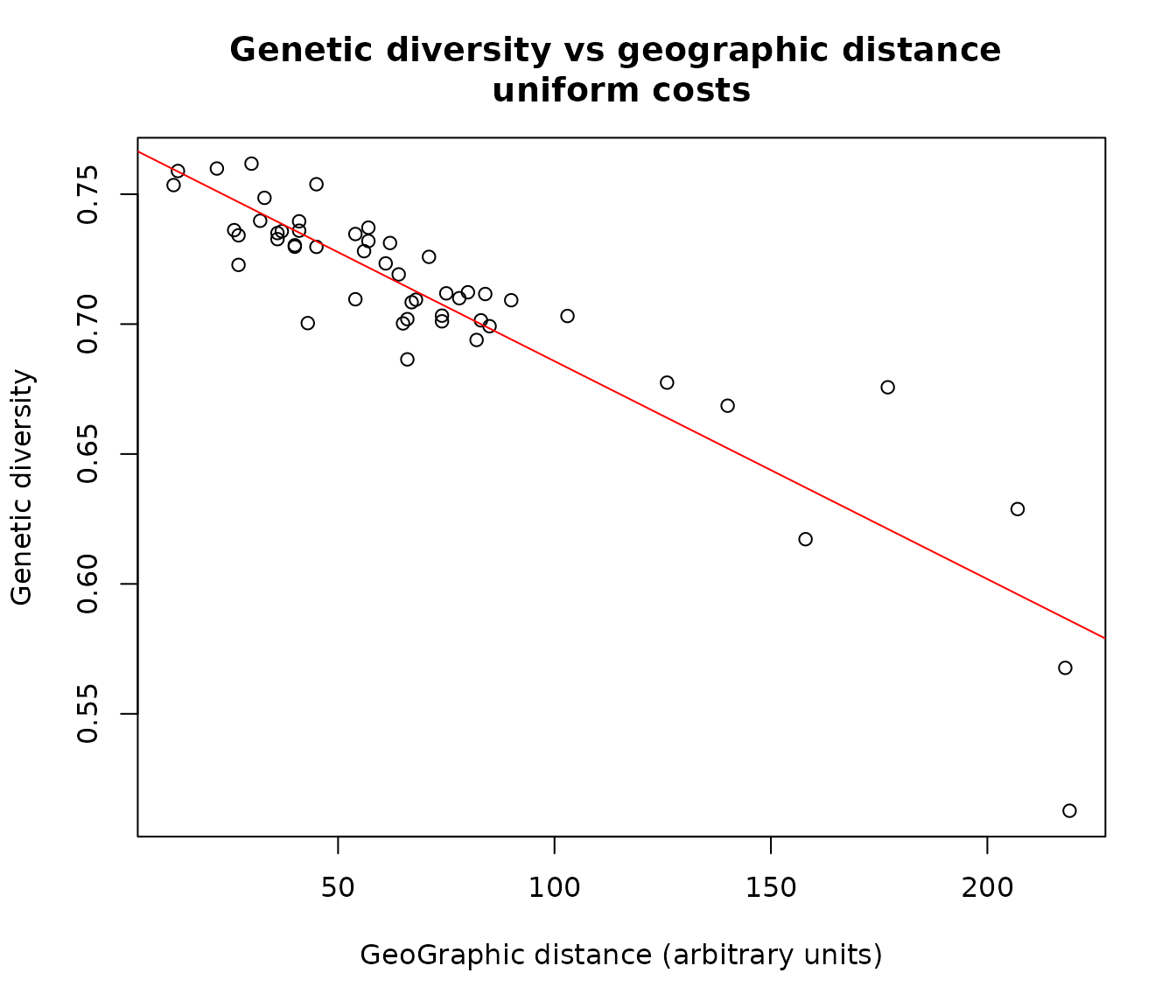

Alternatively, we can use costs based on habitat. As a toy example, we will consider that coasts are four times more favorable for dispersal than the rest of the landmasses. For this we simply use the getCosts function to access the cost-rule data frame and change the cost associated with coastal cells. After defining the new cost rules, we set costs using this data frame with setCosts, and then compute and plot the corresponding shortest paths:

cost.rules <- getCosts(myGraph, res.type = "rules")
cost.rules$cost[cost.rules$habitat == "coast"] <- 0.25

myGraph <- setCosts(myGraph, attr.name = "habitat", cost.rules = cost.rules)
paths.2 <- dijkstraFrom(hgdp, ori)

plot(myGraph, col = NA, reset = TRUE)

## Spherical geometry (s2) switched off

## Spherical geometry (s2) switched on

plot(paths.2)
points(addis[1], addis[2], pch = "x", cex = 2)
text(addis[1] + 35, addis[2], "Addis Ababa", cex = .8, font = 2)
points(hgdp, col.nodes = "black")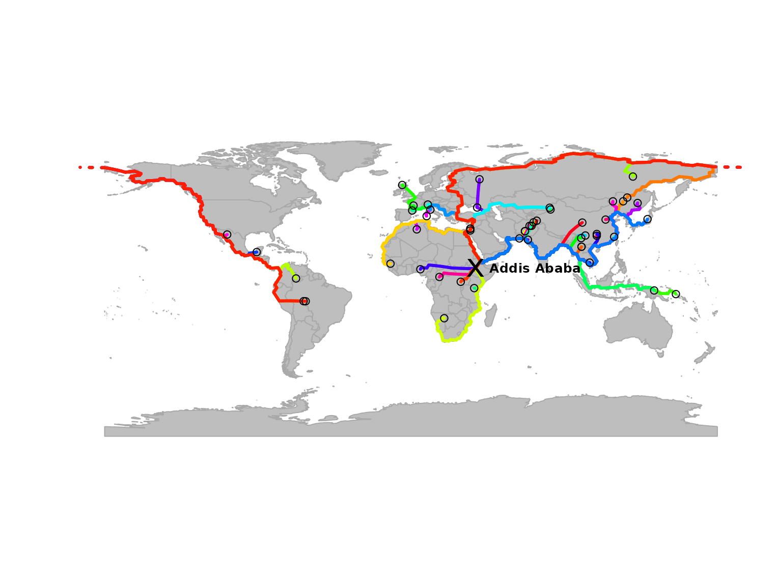

The new paths are slightly different from the previous ones. We can examine the new relationship with genetic distance:

dgeo.hab <- gPath2dist(paths.2)
plot(div ~ dgeo.hab, xlab = "GeoGraphic distance (arbitrary units)", ylab = "Genetic diversity")
lm.hab <- lm(div ~ dgeo.hab)
abline(lm.hab, col = "red")
summary(lm.hab)

## 
## Call:
## lm(formula = div ~ dgeo.hab)
## 
## Residuals:
##      Min       1Q   Median       3Q      Max 
## -0.11182 -0.00993  0.00141  0.01277  0.06413 
## 
## Coefficients:
##              Estimate Std. Error t value Pr(>|t|)    
## (Intercept)  0.770102   0.007282  105.75  < 2e-16 ***
## dgeo.hab    -0.001420   0.000147   -9.69  5.7e-13 ***
## ---
## Signif. codes:  0 '***' 0.001 '**' 0.01 '*' 0.05 '.' 0.1 ' ' 1
## 
## Residual standard error: 0.0268 on 49 degrees of freedom
## Multiple R-squared:  0.657,  Adjusted R-squared:  0.65 
## F-statistic: 93.9 on 1 and 49 DF,  p-value: 5.67e-13

title("Genetic diversity vs geographic distance \n habitat costs ")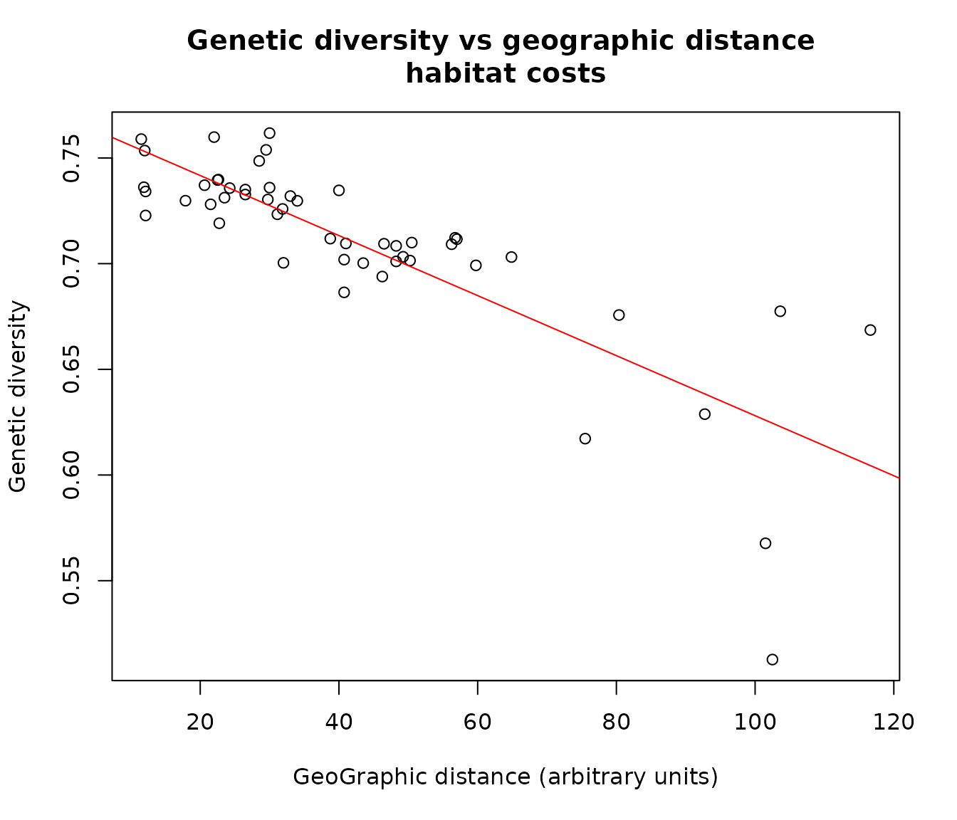

Now of course depending on the application, we may want to use different grid resolutions, and/or more complex habitat information to define costs of traveling through different habitats. This information could for example be incorporated from GIS shapefiles or raster data. Further we maybe also want to edit and customize the gGraph in more detail. This is illustrated in the vignettes ‘Making custom grids’ and ‘Edit graphs’ (see vignette() for more information on available vignettes).