Interpolating Heterozygosity

In this vignette, we will demonstrate how to interpolate measures of genetic diversity across geographic space using the tidypopgen integration with the sf package.

To do so, we will use the Human Genome Diversity Project (HGDP) dataset.

The data files can be downloaded using the following code:

temp_dir <- tempdir()
download_url <-
  "https://zenodo.org/records/17375732/files/hgdp650_id_pop_coords.txt"
download_path <- file.path(temp_dir, "hgdp650_id_pop.txt")
download.file(download_url, download_path, mode = "wb")
download_url <- "https://zenodo.org/records/17375732/files/hgdp650.qc.hg19.bed"
download_path <- file.path(temp_dir, "hgdp650.qc.hg19.bed")
download.file(download_url, download_path, method = "wget")
download_url <- "https://zenodo.org/records/17375732/files/hgdp650.qc.hg19.bim"
download_path <- file.path(temp_dir, "hgdp650.qc.hg19.bim")
download.file(download_url, download_path, method = "wget")
download_url <- "https://zenodo.org/records/17375732/files/hgdp650.qc.hg19.fam"
download_path <- file.path(temp_dir, "hgdp650.qc.hg19.fam")
download.file(download_url, download_path, method = "wget")

Create gen_tibble object

Our first step is to load the HGDP data into a gen_tibble object.

bed_path <- "./data/hgdp/hgdp650.qc.hg19.bed"

hgdp <- gen_tibble(bed_path,
  quiet = TRUE,
  backingfile = tempfile("test_")
)

And add its associated metadata

meta_info <- read_tsv("./data/hgdp/hgdp650_id_pop_coords.txt", col_names = TRUE)
#> Rows: 1043 Columns: 6
#> ── Column specification ───────────────────────────────────────────────────────────────────────────────────
#> Delimiter: "\t"
#> chr (4): id, population, geographic_origin, region
#> dbl (2): latitude, longitude
#> 
#> ℹ Use `spec()` to retrieve the full column specification for this data.
#> ℹ Specify the column types or set `show_col_types = FALSE` to quiet this message.

hgdp <- hgdp %>% mutate(
  population = meta_info$population[match(hgdp$id, meta_info$id)],
  geographic_origin = meta_info$geographic_origin[match(hgdp$id, meta_info$id)],
  region = meta_info$region[match(hgdp$id, meta_info$id)],
  latitude = meta_info$latitude[match(hgdp$id, meta_info$id)],
  longitude = meta_info$longitude[match(hgdp$id, meta_info$id)]
)

Let’s confirm that we have all the expected information:

hgdp
#> # A gen_tibble: 643733 loci
#> # A tibble:     1,043 × 8
#>    id        phenotype  genotypes population geographic_origin            region latitude longitude
#>    <chr>     <fct>     <vctr_SNP> <chr>      <chr>                        <chr>     <dbl>     <dbl>
#>  1 HGDP00448 control    [2,0,...] Biaka_HG   Central_African_Republic     Africa        4        17
#>  2 HGDP00479 control    [1,0,...] Biaka_HG   Central_African_Republic     Africa        4        17
#>  3 HGDP00985 control    [0,0,...] Biaka_HG   Central_African_Republic     Africa        4        17
#>  4 HGDP01094 control    [1,0,...] Biaka_HG   Central_African_Republic     Africa        4        17
#>  5 HGDP00982 control    [2,0,...] Mbuti_HG   Democratic_Republic_of_Congo Africa        1        29
#>  6 HGDP00911 control    [1,0,...] Mandenka   Senegal                      Africa       12       -12
#>  7 HGDP01202 control    [2,0,...] Mandenka   Senegal                      Africa       12       -12
#>  8 HGDP00927 control    [2,0,...] Yoruba     Nigeria                      Africa        8         5
#>  9 HGDP00461 control    [2,0,...] Biaka_HG   Central_African_Republic     Africa        4        17
#> 10 HGDP00451 control    [2,0,...] Biaka_HG   Central_African_Republic     Africa        4        17
#> # ℹ 1,033 more rows

Gen_tibble with sf

Now that we have latitudes and longitudes in our tibble; we can transform them into an sf geometry with the function gt_add_sf(). Once we have done that, our gen_tibble will act as an sf object, which can be plotted with ggplot2.

hgdp <- gt_add_sf(hgdp, c("longitude", "latitude"))
hgdp
#> Simple feature collection with 1043 features and 8 fields
#> Geometry type: POINT
#> Dimension:     XY
#> Bounding box:  xmin: -108 ymin: -25.83333 xmax: 155 ymax: 63
#> Geodetic CRS:  WGS 84
#> # A gen_tibble: 643733 loci
#> # A tibble:     1,043 × 9
#>    id        phenotype  genotypes population geographic_origin            region latitude longitude
#>    <chr>     <fct>     <vctr_SNP> <chr>      <chr>                        <chr>     <dbl>     <dbl>
#>  1 HGDP00448 control    [2,0,...] Biaka_HG   Central_African_Republic     Africa        4        17
#>  2 HGDP00479 control    [1,0,...] Biaka_HG   Central_African_Republic     Africa        4        17
#>  3 HGDP00985 control    [0,0,...] Biaka_HG   Central_African_Republic     Africa        4        17
#>  4 HGDP01094 control    [1,0,...] Biaka_HG   Central_African_Republic     Africa        4        17
#>  5 HGDP00982 control    [2,0,...] Mbuti_HG   Democratic_Republic_of_Congo Africa        1        29
#>  6 HGDP00911 control    [1,0,...] Mandenka   Senegal                      Africa       12       -12
#>  7 HGDP01202 control    [2,0,...] Mandenka   Senegal                      Africa       12       -12
#>  8 HGDP00927 control    [2,0,...] Yoruba     Nigeria                      Africa        8         5
#>  9 HGDP00461 control    [2,0,...] Biaka_HG   Central_African_Republic     Africa        4        17
#> 10 HGDP00451 control    [2,0,...] Biaka_HG   Central_African_Republic     Africa        4        17
#> # ℹ 1,033 more rows
#> # ℹ 1 more variable: geometry <POINT [°]>

library(spData)
library(sf)
library(terra)
library(tmap)
library(viridis)

Calculating heterozygosity is simple in tidypopgen. First, lets run some basic filtering to remove SNPs in linkage:

hgdp <- gt_impute_simple(hgdp)
to_keep <- hgdp %>% loci_ld_clump(
  thr_r2 = 0.2, size = 100,
  return_id = TRUE, use_positions = TRUE
)
hgdp <- hgdp %>% select_loci(all_of(to_keep))

We can store heterozygosity for each individual in our gen_tibble object by creating a column with mutate() and using the function indiv_het_obs() to calculate observed heterozygosity for each individual. Then we can create a new column with the mean heterozygosity for each population

hgdp <- hgdp %>% mutate(heterozygosity = indiv_het_obs(genotypes))
mean_het <- hgdp %>%
  group_by(population) %>%
  summarise(mean_het = mean(heterozygosity))
hgdp <-
  hgdp %>%
  mutate(mean_het = mean_het$mean_het[match(
    hgdp$population,
    mean_het$population
  )])

We can then begin by creating a global map using rnaturalearth.

library(rnaturalearth)

map <- ne_countries(scale = "medium") %>%
  filter(sovereignt != "Antarctica")
map <- st_union(map) %>% st_sf()
map <- st_cast(map, "POLYGON")
map <- st_wrap_dateline(map, options = c("WRAPDATELINE=YES"))

We can check the distribution of our samples across the map using our gen_tibble with sf geometry:

ggplot() +
  geom_sf(data = hgdp$geometry) +
  geom_sf(data = map, fill = NA) +
  theme_minimal()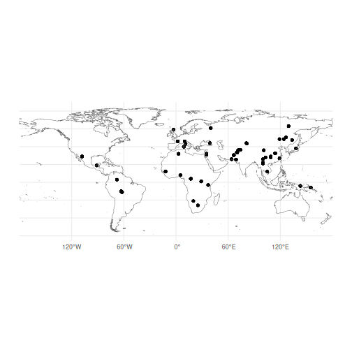

plot of chunk hgdp_map

Our map shows the distribution of the HGDP data, but we can see that there are gaps in the sampling. We know that heterozygosity decreases with distance from Africa, so we can use spatial interpolation to estimate heterozygosity in unsampled areas.

To begin, we will create a grid of points covering the map.

grid <- rast(map, nrows = 200, ncols = 200)
xy <- xyFromCell(grid, 1:ncell(grid))

By converting this grid to an sf object, we can then use st_filter() to keep only the points that fall within the landmasses.

coop <- st_as_sf(as.data.frame(xy),
  coords = c("x", "y"),
  crs = st_crs(map)
)
coop <- st_filter(coop, map)

And we can quickly visualise this grid using the qtm autoplotting function from the tmap package:

qtm(coop)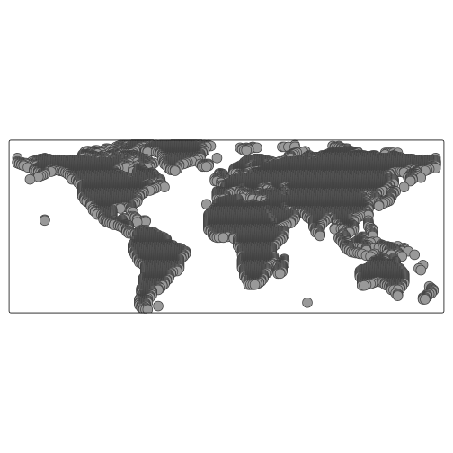

plot of chunk global_grid_map

Now we can use the gstat package to perform spatial interpolation of heterozygosity.

gstat implements several methods for spatial interpolation, including inverse distance weighting (IDW) and kriging. Here, we will use IDW to interpolate heterozygosity across our grid of points.

We remove the genotypes from our gen_tibble, as gstat does not accept a gen_tibble object, and then run the interpolation:

hgdp_sf_obj <- hgdp %>% select(-"genotypes")

library(gstat)
res <- gstat(
  formula = mean_het ~ 1, locations = hgdp_sf_obj,
  nmax = nrow(hgdp_sf_obj),
  set = list(idp = 1)
)

resp <- predict(res, coop)
#> [inverse distance weighted interpolation]
resp$x <- st_coordinates(resp)[, 1]
resp$y <- st_coordinates(resp)[, 2]

We can visualise the interpolated values using tmap:

pred <- rasterize(resp, grid, field = "var1.pred", fun = "mean")
tm_shape(pred) + tm_raster(alpha = 0.6, palette = "viridis")
#> 
#> ── tmap v3 code detected ──────────────────────────────────────────────────────────────────────────────────
#> [v3->v4] `tm_tm_raster()`: migrate the argument(s) related to the scale of the visual variable `col`
#> namely 'palette' (rename to 'values') to col.scale = tm_scale(<HERE>).
#> [v3->v4] `tm_raster()`: use `col_alpha` instead of `alpha`.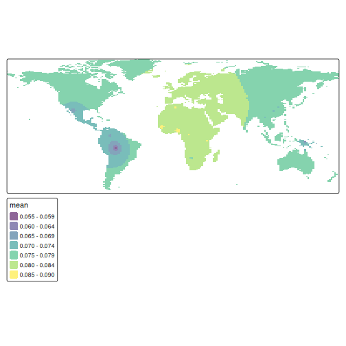

plot of chunk interpolated_map

Or, for a more publication-ready figure, we can use ggplot2 and the tidyterra package:

library(tidyterra)

ggplot() +
  geom_sf(data = hgdp, aes(colour = mean_het)) +
  geom_spatraster(data = pred, aes(fill = var1.pred)) +
  scale_fill_viridis_c(
    name = "Interpolated Heterozygosity",
    alpha = 0.8,
    na.value = NA
  ) +
  scale_color_viridis_c(name = "Observed", alpha = 0.8) +
  theme_minimal()
#> Error in `geom_spatraster()`:
#> ! Problem while computing aesthetics.
#> ℹ Error occurred in the 2nd layer.
#> Caused by error:
#> ! object 'var1.pred' not found

Interpolating Heterozygosity

2025-10-14

Create gen_tibble object

Gen_tibble with sf

Interpolating heterozygosity