Site frequency spectra • tidypopgen

The site frequency spectrum (SFS) counts the number of sites at which an allele is found in 1, 2, 3, … copies in a sample. Joint spectra do the same for several populations at once. They are the input of demographic inference with dadi, moments or fastsimcoal2.

The main difficulty with real data is missing genotypes: different sites are genotyped in a different number of individuals. tidypopgen deals with them as easySFS does. Each population is projected down to a fixed number of allele copies, by computing for every site the probability of each allele count in a random subsample of that size. Sites with fewer genotyped copies are dropped. This article shows the whole workflow:

choosing the projection;
computing and plotting the spectra;
estimating their uncertainty with a block bootstrap;
exporting them for dadi and fastsimcoal2.

The data

We use the RAD-seq data of Anolis punctatus lizards shipped with the package (see the vignette ‘Population genetic analysis with tidypopgen’). We group the 46 individuals into three populations: the Atlantic Forest (AF), and the eastern (Eam) and western (Wam) Amazonian Forest.

library(tidypopgen)
#> Loading required package: dplyr
#> 
#> Attaching package: 'dplyr'
#> The following objects are masked from 'package:stats':
#> 
#>     filter, lag
#> The following objects are masked from 'package:base':
#> 
#>     intersect, setdiff, setequal, union
#> Loading required package: tibble
vcf_path <-
  system.file("/extdata/anolis/punctatus_t70_s10_n46_filtered.recode.vcf.gz",
    package = "tidypopgen"
  )
anole_gt <-
  gen_tibble(vcf_path, quiet = TRUE, backingfile = tempfile("anolis_"))
pops_path <- system.file("/extdata/anolis/punctatus_n46_meta.csv",
  package = "tidypopgen"
)
pops <- read.csv(pops_path)
anole_gt <- anole_gt %>%
  left_join(pops, by = "id") %>%
  group_by(pop)

As usual for RAD-seq data, many genotypes are missing. loci_missingness() gives the proportion of missing genotypes at each SNP in each population. Only 4 to 10% of the genotypes are missing (mean_missing), but they are spread over many SNPs: in the two Amazonian populations, about two thirds of the SNPs are missing in at least one individual (prop_snps_missing):

anole_gt %>%
  loci_missingness(type = "tidy") %>%
  group_by(group) %>%
  summarise(
    mean_missing = mean(value),
    prop_snps_missing = mean(value > 0)
  )
#> # A tibble: 3 × 3
#>   group mean_missing prop_snps_missing
#>   <chr>        <dbl>             <dbl>
#> 1 AF          0.0412             0.231
#> 2 Eam         0.0811             0.660
#> 3 Wam         0.0965             0.655

SNPs found on the same RAD locus are tightly linked. By default, easySFS keeps a single random SNP per RAD locus. Here the RAD loci are recorded as chromosomes, so we do the same with select_loci():

set.seed(123)
one_per_locus <- show_loci(anole_gt) %>%
  mutate(index = row_number()) %>%
  group_by(chromosome) %>%
  slice_sample(n = 1) %>%
  pull(index)
anole_thin <- anole_gt %>% select_loci(all_of(sort(one_per_locus)))
count_loci(anole_thin)
#> [1] 1920

Choosing the projection

Projecting to more allele copies gives a finer spectrum, with more rare variants, but drops more sites with missing data. pop_sfs_preview(), the equivalent of easySFS --preview, gives the number of segregating sites for each possible projection of each population:

preview <- pop_sfs_preview(anole_thin)
autoplot(preview)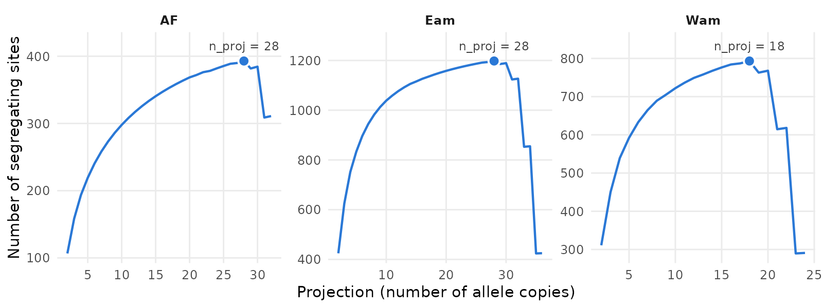

Following the dadi manual, a good choice maximises the number of segregating sites. The best column marks that projection for each population, which is what all the SFS functions use when n_proj is not given:

preview %>% filter(best)
#> # A tibble: 3 × 5
#>   group n_proj n_seg_sites n_loci best 
#>   <chr>  <int>       <dbl>  <dbl> <lgl>
#> 1 AF        28        393.   1862 TRUE 
#> 2 Eam       28       1198.   1869 TRUE 
#> 3 Wam       18        793.   1859 TRUE

One-dimensional spectra

pop_sfs() computes the spectrum of each population. As n_proj is not given, a message reports the projections it chose:

sfs_1d <- pop_sfs(anole_thin)
#> `n_proj` not given; each group is projected to the number of allele copies that maximises its number of segregating sites (see pop_sfs_preview()): AF = 28, Eam = 28, Wam = 18
sfs_1d
#> # A tibble: 77 × 4
#>    group allele_count n_sites masked
#>    <chr>        <int>   <dbl> <lgl> 
#>  1 AF               0  1469.  TRUE  
#>  2 AF               1    83.8 FALSE 
#>  3 AF               2    60.0 FALSE 
#>  4 AF               3    46.3 FALSE 
#>  5 AF               4    35.1 FALSE 
#>  6 AF               5    24.6 FALSE 
#>  7 AF               6    23.0 FALSE 
#>  8 AF               7    19.0 FALSE 
#>  9 AF               8    18.5 FALSE 
#> 10 AF               9    20.0 FALSE 
#> # ℹ 67 more rows
autoplot(sfs_1d)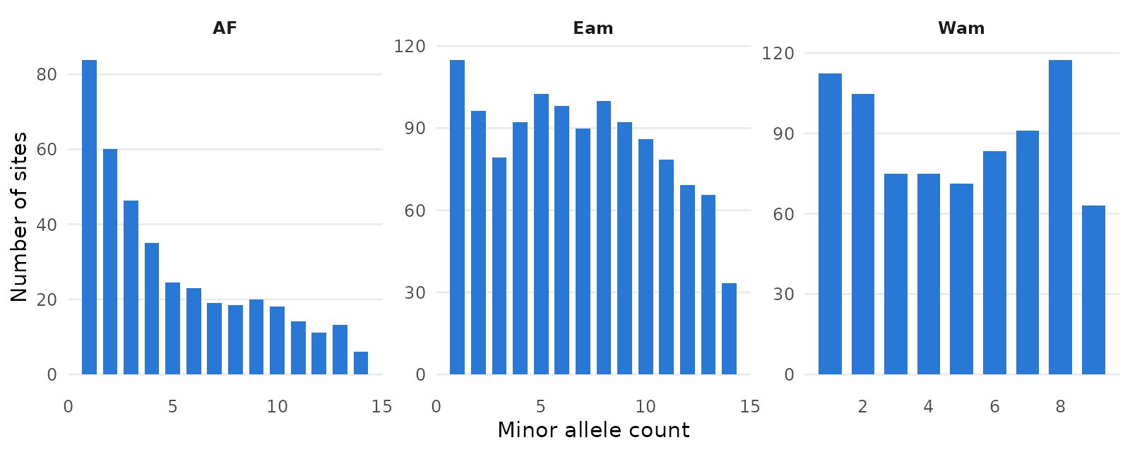

The spectra are folded by default (they count copies of the minor allele), as the ancestral allele is rarely known. With folded = FALSE, the reference allele is taken to be ancestral (as in easySFS). You can also give the ancestral allele of each locus, e.g. from an outgroup, with ancestral. The output is a tidy tibble, with the projections stored in its n_proj attribute.

The cells with no copies of the minor allele (sites monomorphic in the projected sample), and those folded out, are masked (as in dadi). They are not plotted by default.

Joint spectra

pairwise_pop_sfs() computes the joint spectrum of each pair of populations. Each spectrum only uses the sites with enough genotyped copies in both of its populations. It is plotted as a heatmap, on a log scale:

n_proj <- attr(sfs_1d, "n_proj")
sfs_2d <- pairwise_pop_sfs(anole_thin, n_proj = n_proj)
autoplot(sfs_2d)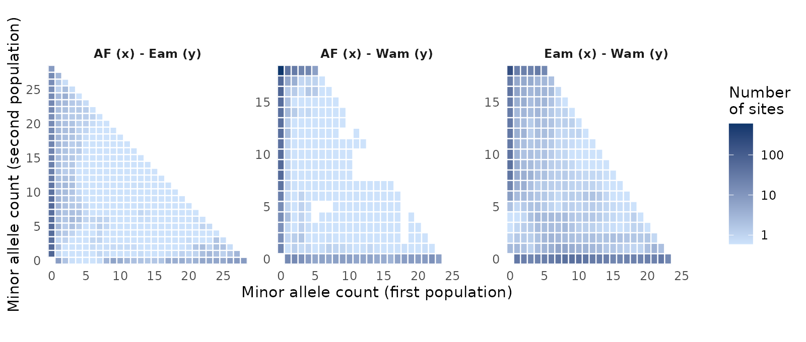

In all three pairs, most sites lie along the axes: their minor allele is found in only one of the two populations. The bottom row holds the variants of the first population that are absent from the second, and the left column those of the second population. The top left corner holds sites where the minor allele (across the pair) is common in the second population but rare in the first. The interior, where the two populations share variants at intermediate frequencies, holds fewer sites, and fewest in the two pairs that include the Atlantic Forest.

nwise_pop_sfs() computes the joint spectrum of all populations. Its cells are listed in the order of the populations, with the last one changing fastest (use fastest = "first" for the opposite order):

sfs_3d <- nwise_pop_sfs(anole_thin, n_proj = n_proj)
sfs_3d
#> # A tibble: 15,979 × 5
#>       AF   Eam   Wam       n_sites masked
#>    <int> <int> <int>         <dbl> <lgl> 
#>  1     0     0     0  0.0000000719 TRUE  
#>  2     0     0     1  0.00000284   FALSE 
#>  3     0     0     2  0.0000732    FALSE 
#>  4     0     0     3  0.00534      FALSE 
#>  5     0     0     4  0.122        FALSE 
#>  6     0     0     5  1.27         FALSE 
#>  7     0     0     6  6.63         FALSE 
#>  8     0     0     7 20.1          FALSE 
#>  9     0     0     8 35.9          FALSE 
#> 10     0     0     9 42.6          FALSE 
#> # ℹ 15,969 more rows

With type = "array", all these functions return arrays (sfs objects) instead of tibbles.

Uncertainty: block bootstrap

bootstrap_pop_sfs(), bootstrap_pairwise_pop_sfs() and bootstrap_nwise_pop_sfs() resample blocks of loci with replacement. The blocks are defined as in the jackknife_* functions: SNPs, base pairs or centiMorgans, never spanning two chromosomes. Blocks should be larger than the extent of linkage disequilibrium. Here we kept a single SNP per RAD locus, and RAD loci are not mapped, so we resample single SNPs (block_size = 1):

set.seed(42)
boot <- bootstrap_pop_sfs(anole_thin,
  n_bootstrap = 100, block_size = 1,
  n_proj = n_proj
)
boot
#> # A tibble: 7,700 × 5
#>    group replicate allele_count n_sites masked
#>    <chr>     <int>        <int>   <dbl> <lgl> 
#>  1 AF            1            0  1438.  TRUE  
#>  2 AF            1            1    90.6 FALSE 
#>  3 AF            1            2    65.8 FALSE 
#>  4 AF            1            3    47.5 FALSE 
#>  5 AF            1            4    26.7 FALSE 
#>  6 AF            1            5    21.2 FALSE 
#>  7 AF            1            6    24.9 FALSE 
#>  8 AF            1            7    20.4 FALSE 
#>  9 AF            1            8    20.9 FALSE 
#> 10 AF            1            9    24.8 FALSE 
#> # ℹ 7,690 more rows

The genotypes are read only once, whatever the number of replicates. We can then add a 95% interval to each cell of the spectra:

library(ggplot2)
boot_ci <- boot %>%
  filter(!masked) %>%
  group_by(group, allele_count) %>%
  summarise(
    lower = quantile(n_sites, 0.025),
    upper = quantile(n_sites, 0.975),
    .groups = "drop"
  )
sfs_1d %>%
  filter(!masked) %>%
  left_join(boot_ci, by = c("group", "allele_count")) %>%
  ggplot(aes(x = allele_count, y = n_sites)) +
  geom_col(fill = "#2a78d6", width = 0.7) +
  geom_errorbar(aes(ymin = lower, ymax = upper),
    width = 0.3, colour = "grey30"
  ) +
  # integer breaks for allele counts
  scale_x_continuous(breaks = function(x) unique(floor(pretty(x)))) +
  facet_wrap(~group, scales = "free") +
  labs(x = "Minor allele count", y = "Number of sites") +
  theme_minimal()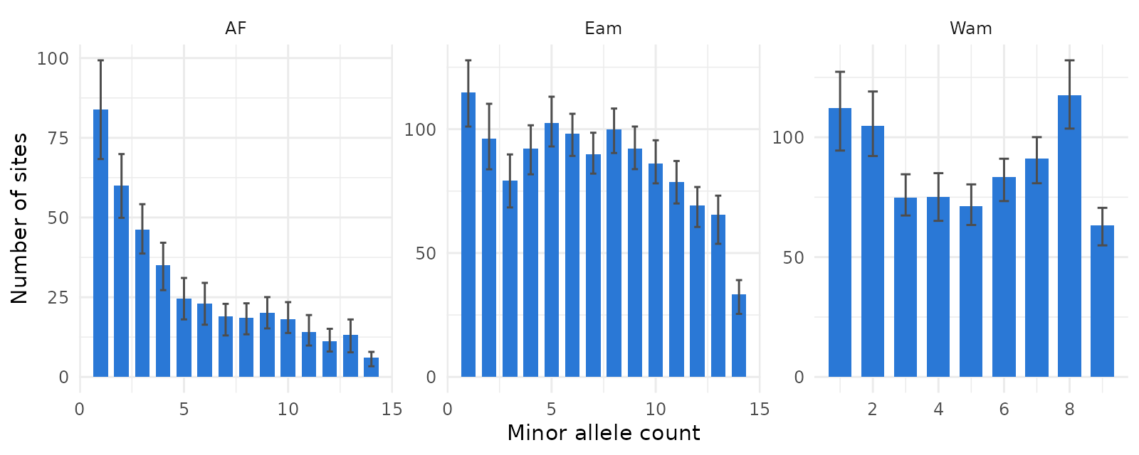

Exporting to dadi and fastsimcoal2

write_sfs() writes spectra in the formats of dadi (format = "dadi") and fastsimcoal2 (format = "fastsimcoal2"). Given a grouped gen_tibble, it writes all the spectra that easySFS writes, in a single pass over the genotypes: - the 1D spectrum of each population; - the joint spectrum of each pair; - the joint spectrum of all populations.

They have the same file names as in easySFS. Writing each format to the dadi and fastsimcoal2 sub-directories of a folder gives the layout of easySFS:

out_dir <- file.path(tempdir(), "anolis_sfs")
dadi_files <- write_sfs(anole_thin,
  out_dir = file.path(out_dir, "dadi"),
  n_proj = n_proj
)
basename(dadi_files)
#> [1] "AF-28.sfs"      "Eam-28.sfs"     "Wam-18.sfs"     "AF-Eam.sfs"    
#> [5] "AF-Wam.sfs"     "Eam-Wam.sfs"    "AF-Eam-Wam.sfs"

With n_bootstrap, it also writes each bootstrap replicate in its own sub-directory, e.g. to estimate confidence intervals of the parameters fitted with fastsimcoal2:

fastsimcoal2_files <- write_sfs(anole_thin,
  out_dir = file.path(out_dir, "fastsimcoal2"), format = "fastsimcoal2",
  n_proj = n_proj, prefix = "anolis",
  n_bootstrap = 10, bootstrap_block_size = 1
)
list.files(file.path(out_dir, "fastsimcoal2"))
#>  [1] "AF_MAFpop0.obs"            "anolis_jointMAFpop1_0.obs"
#>  [3] "anolis_jointMAFpop2_0.obs" "anolis_jointMAFpop2_1.obs"
#>  [5] "anolis_MSFS.obs"           "bootstrap_01"             
#>  [7] "bootstrap_02"              "bootstrap_03"             
#>  [9] "bootstrap_04"              "bootstrap_05"             
#> [11] "bootstrap_06"              "bootstrap_07"             
#> [13] "bootstrap_08"              "bootstrap_09"             
#> [15] "bootstrap_10"              "Eam_MAFpop0.obs"          
#> [17] "Wam_MAFpop0.obs"
list.files(file.path(out_dir, "fastsimcoal2", "bootstrap_01"))
#> [1] "AF_MAFpop0.obs"            "anolis_jointMAFpop1_0.obs"
#> [3] "anolis_jointMAFpop2_0.obs" "anolis_jointMAFpop2_1.obs"
#> [5] "anolis_MSFS.obs"           "Eam_MAFpop0.obs"          
#> [7] "Wam_MAFpop0.obs"

Given a single spectrum (an sfs object, returned with type = "array"), write_sfs() writes it to a file. Here we write the spectrum of the western Amazonian population. We round its cells to integers (round = TRUE, as easySFS --dtype int) to make the file easier to read:

sfs_wam <- pop_sfs(anole_thin, n_proj = n_proj, type = "array")$Wam
dadi_file <- tempfile(fileext = ".sfs")
write_sfs(sfs_wam, dadi_file, format = "dadi", round = TRUE)
writeLines(readLines(dadi_file))
#> 19 folded "Wam"
#> 1066 112 105 75 75 71 83 91 117 63 0 0 0 0 0 0 0 0 0
#> 1 0 0 0 0 0 0 0 0 0 1 1 1 1 1 1 1 1 1

A dadi file has three lines:

the number of cells (the number of allele copies plus 1), whether the spectrum is folded, and the population label;
the number of sites with 0, 1, 2, … copies of the minor allele;
the mask: 1 for the masked cells, which are the cell with no copies of the minor allele and the cells with more than half of the copies (which are folded out).

For a joint spectrum, the first line gives the number of cells and the label of each population. The second line lists the cells with the number of copies in the last population changing fastest.

The first cell (no copies of the minor allele in the projected sample) only counts the SNPs in the gen_tibble that are monomorphic in this population. It does not count the sites that were sequenced but are not SNPs. dadi masks this cell. fastsimcoal2 uses it as the number of monomorphic sites, to estimate parameters in absolute units (e.g. effective population sizes, given a mutation rate). If you know the total number of sites sequenced, total_length sets the first cell to that number minus the sites in all the other cells, as easySFS --total-length does. If the SNPs have been thinned, as here, where we kept one SNP per RAD locus, scale the total length by the proportion of SNPs kept (the number of SNPs after thinning over the number before), so that monomorphic sites are sampled at the same rate as SNPs. The Anolis data shipped with the package do not record the number of sites sequenced, so here we use a made-up total length of 100,000 sites before thinning, scaled by the proportion of SNPs we kept:

total_length <- 100000 * count_loci(anole_thin) / count_loci(anole_gt)
total_length
#> [1] 59095.11
fastsimcoal2_file <- tempfile(fileext = "_MAFpop0.obs")
write_sfs(sfs_wam, fastsimcoal2_file,
  format = "fastsimcoal2",
  total_length = total_length, round = TRUE
)
writeLines(readLines(fastsimcoal2_file))
#> 1 observation
#> d0_0 d0_1    d0_2    d0_3    d0_4    d0_5    d0_6    d0_7    d0_8    d0_9    d0_10   d0_11   d0_12   d0_13   d0_14   d0_15   d0_16   d0_17   d0_18
#> 58302 112 105 75 75 71 83 91 117 63 0 0 0 0 0 0 0 0 0

In the fastsimcoal2 file, the first line gives the number of observed spectra, and the second labels the cells. The first cell now holds the scaled total length minus the sites in the other cells, which are unchanged. total_length can also be given to write_sfs() for a gen_tibble, to set the first cell of all the spectra it writes.